- resolution differences between devices (e.g. the on-screen device vs. file device)
- absolute vs. relative sizing of elements
EDS 240: Discussion 6
Saving plots
Week 6 | February 11th, 2025
Where we left off . . .
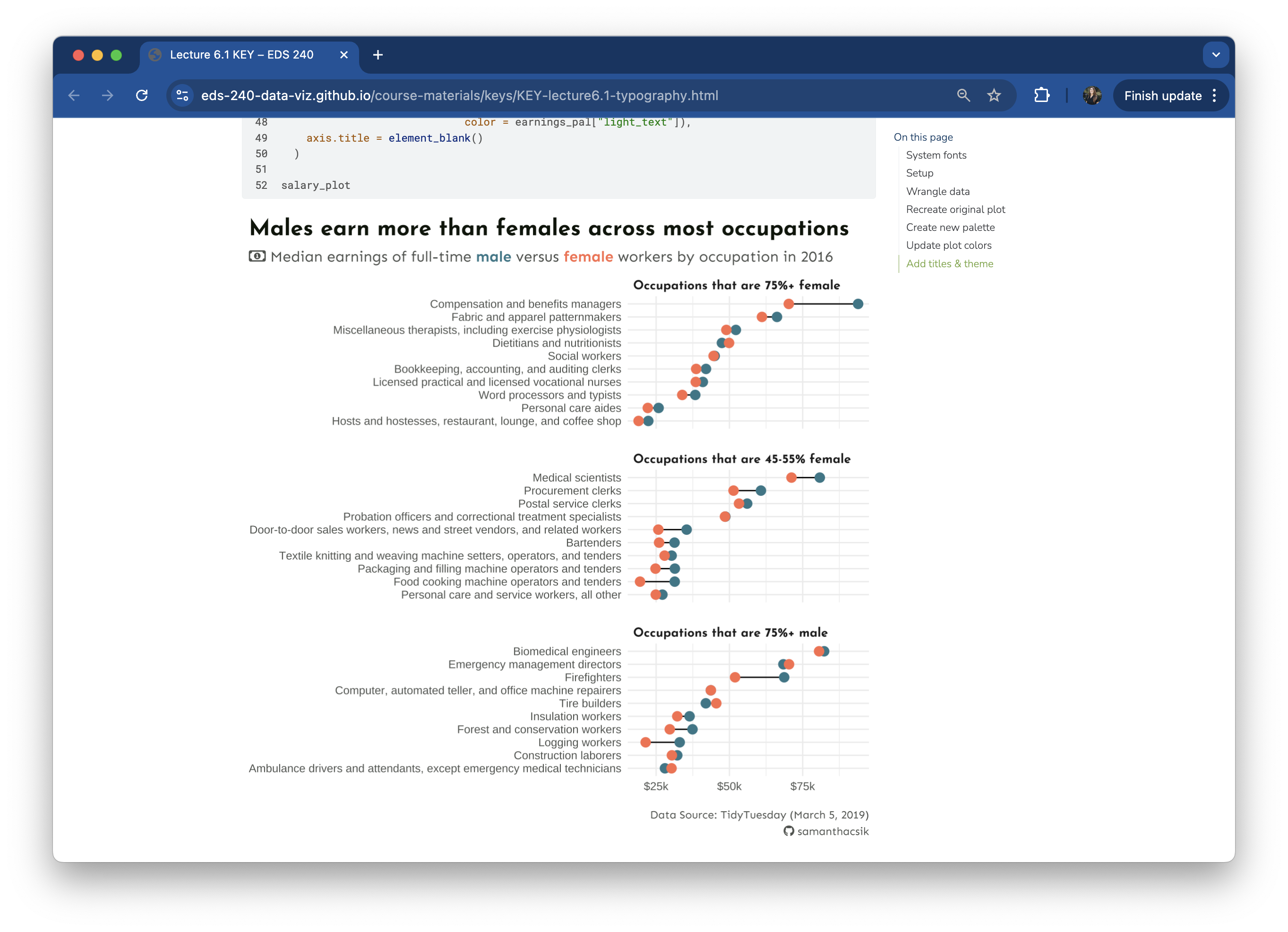
We iterated on our salary plot by updating colors, theme elements, and most notably, our fonts. It rendered nicely in our Quarto doc, with the help of a couple code chunk options to set the size (out-width: "100%") and aspect ratio (fig-asp: 1):
Where we left off . . .
However, when we tried saving our plot as a PNG file using ggsave(), we got something that looked quite different:
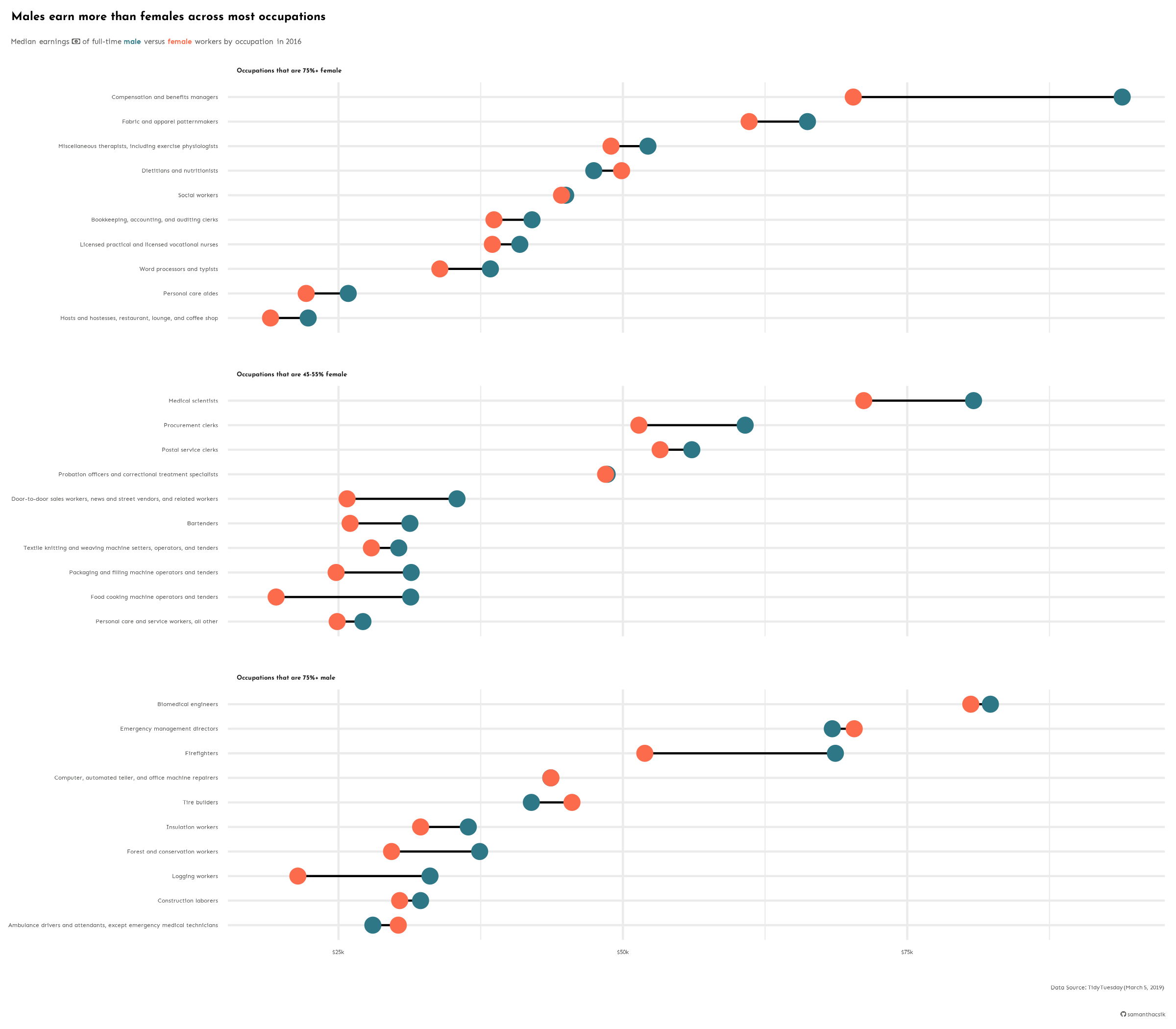
Text scaling can be challenging
There are a number of reasons why, but two big ones:
NOTE: Your computer’s screen resolution may be different than mine. If you’re plot doesn’t appear exactly as mine does (either when plotted on-screen, or saved as a file), this might be why! You may need to tweak some sizes so that your plot looks as it should.
Issue #1: resolution differences between devices
Some definitions first
Digital image size is described in pixel (px) dimensions (e.g. 2400 x 2100 px). A pixel is a basic (and smallest) unit of programmable color on a computer display. To calculate pixel dimensions, we need to know:
- the width of the image (e.g. 8 inches – we’ve defined this is
ggsave()) - the height of the image (e.g. 7 inches – we’ve also defined this is
ggsave()) - the resolution of the image (in pixels per inch, e.g. 300 PPI)
pixel dimensions = \((8"W \times 300\:PPI) \times (7"H \times 300\:PPI) = 2400 \times 2100\:px\)
Image source: What are ‘Image Size’ and ‘Resolution’?
For us, PPI == DPI
Printed image resolution is represented as dots per inch (DPI), which refers to the literal printed dots of ink per inch. While PPI and DPI are technically different, they are often used interchangeably and the conversion is generally taken as 1 PPI : 1 DPI. We will use PPI and DPI interchangeably.
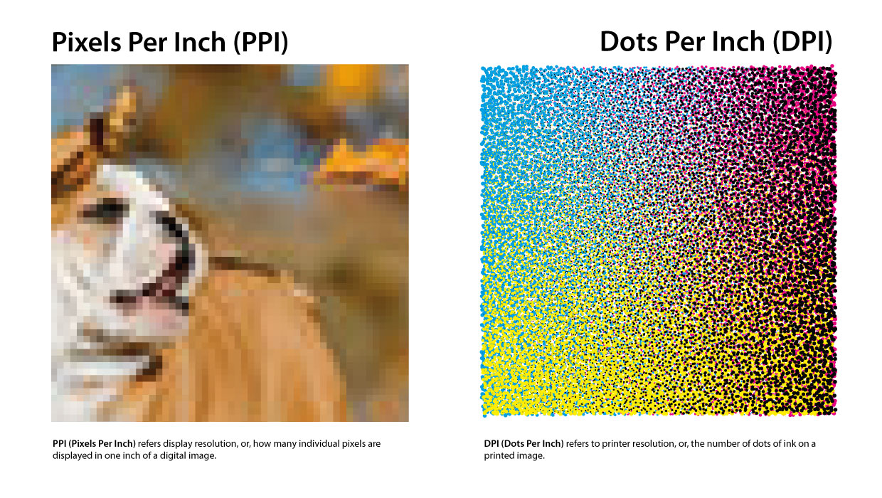
Image source: What is DPI?
Make sure {showtext} and ggsave() DPIs match
By default, {showtext} uses a resolution of 96 DPI when rendering our plot on screen, while ggsave() uses a default resolution of 300 DPI to write our plot to file. This mismatch is one major cause of inconsistent font renderings across different devices. Ensure that these match:
- Set the
{showtext}DPI (best to do this at the top of your script):
- (Optional) Set the DPI in
ggsave()(300 is the default, so this step is optional):
An image is generally considered “high-resolution” if it has 300+ PPI. The conversion of PPI to DPI is usually 1:1, we’ll set a DPI of 300 for both {showtext} and ggsave().
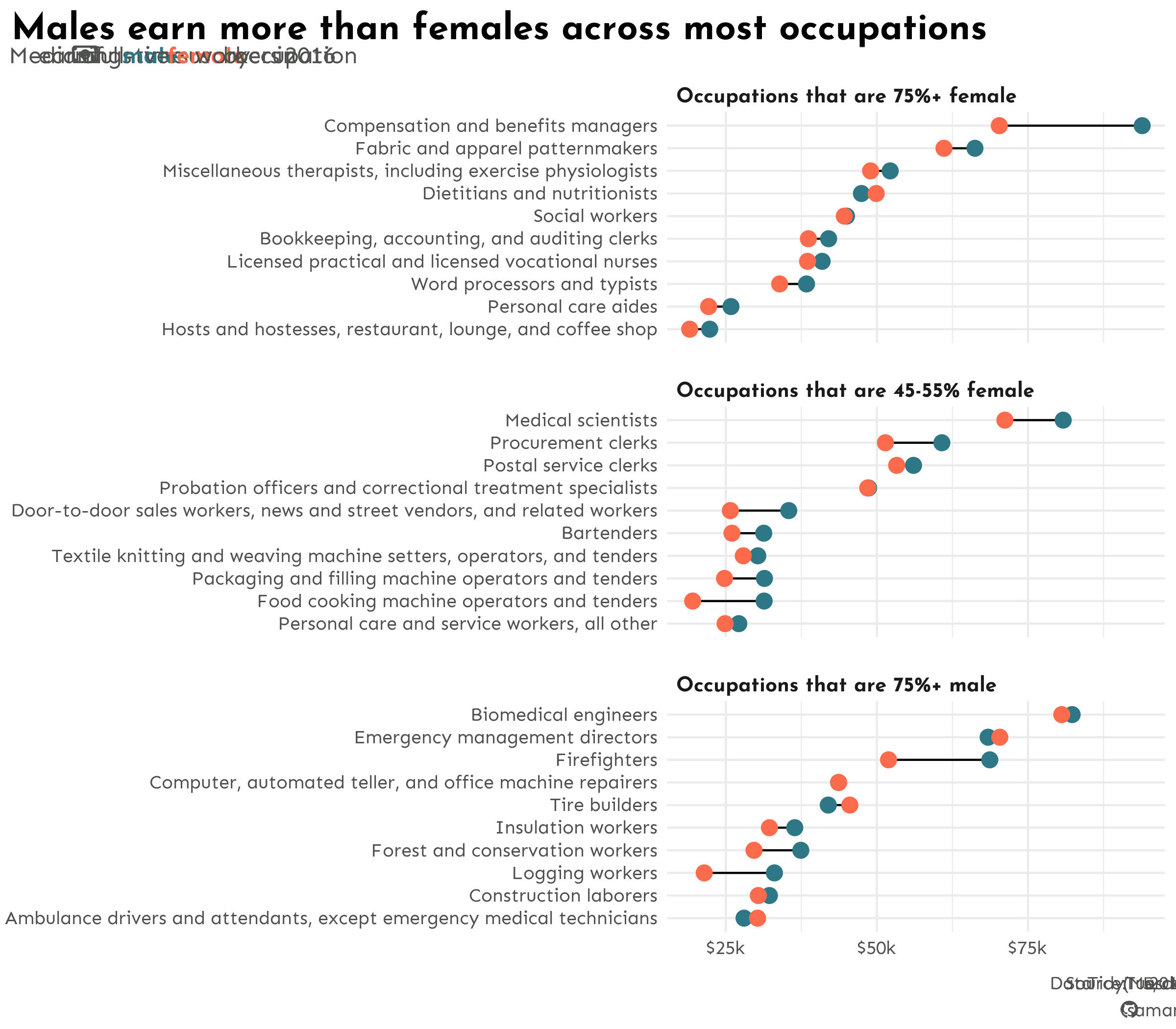
That largely took care of our font sizing issue! But our {ggtext} elements look super wonky…
Issue #2: absolute vs relative sizes of elements
{ggtext} elements rely on absolute units
{ggtext} deals in absolute units (e.g. in, cm), which means elements (e.g. element_textbox()) don’t scale dynamically with plot size. Let’s temporarily fill our element_textbox()es with color to help visualize this:
updated_plot <- plot +
  labs(title = "Males earn more than females across most occupations",
       subtitle = subtitle,
       caption = caption) +
  theme_minimal() +
  theme(
    plot.title.position = "plot",
    plot.title = element_text(family = "josefin",
                              face = "bold",
                              size = 18),
    plot.subtitle = ggtext::element_textbox(family = "sen",
                                            size = 12,
                                            color = earnings_pal["light_text"],
                                            fill = "lightblue", # for debugging
                                            margin = margin(t = 2, r = 0, b = 6, l = 0)),
    plot.caption = ggtext::element_textbox(family = "sen",
                                           face = "italic", # NOTE: this no longer applies since the typeface "sen" does not exist in an italic font style
                                           color = earnings_pal["light_text"],
                                           fill = "lightblue", # for debugging
                                           halign = 1,
                                           lineheight = 1.5,
                                           margin = margin(t = 15, r = 0, b = 0, l = 0)),
    strip.text.x = element_text(family = "josefin",
                                face = "bold",
                                size = 10,
                                hjust = 0),
    panel.spacing.y = unit(0.5, "cm"),
    axis.text = element_text(family = "sen",
                             size = 9,
                             color = earnings_pal["light_text"]),
    axis.title = element_blank()
  )

updated_plot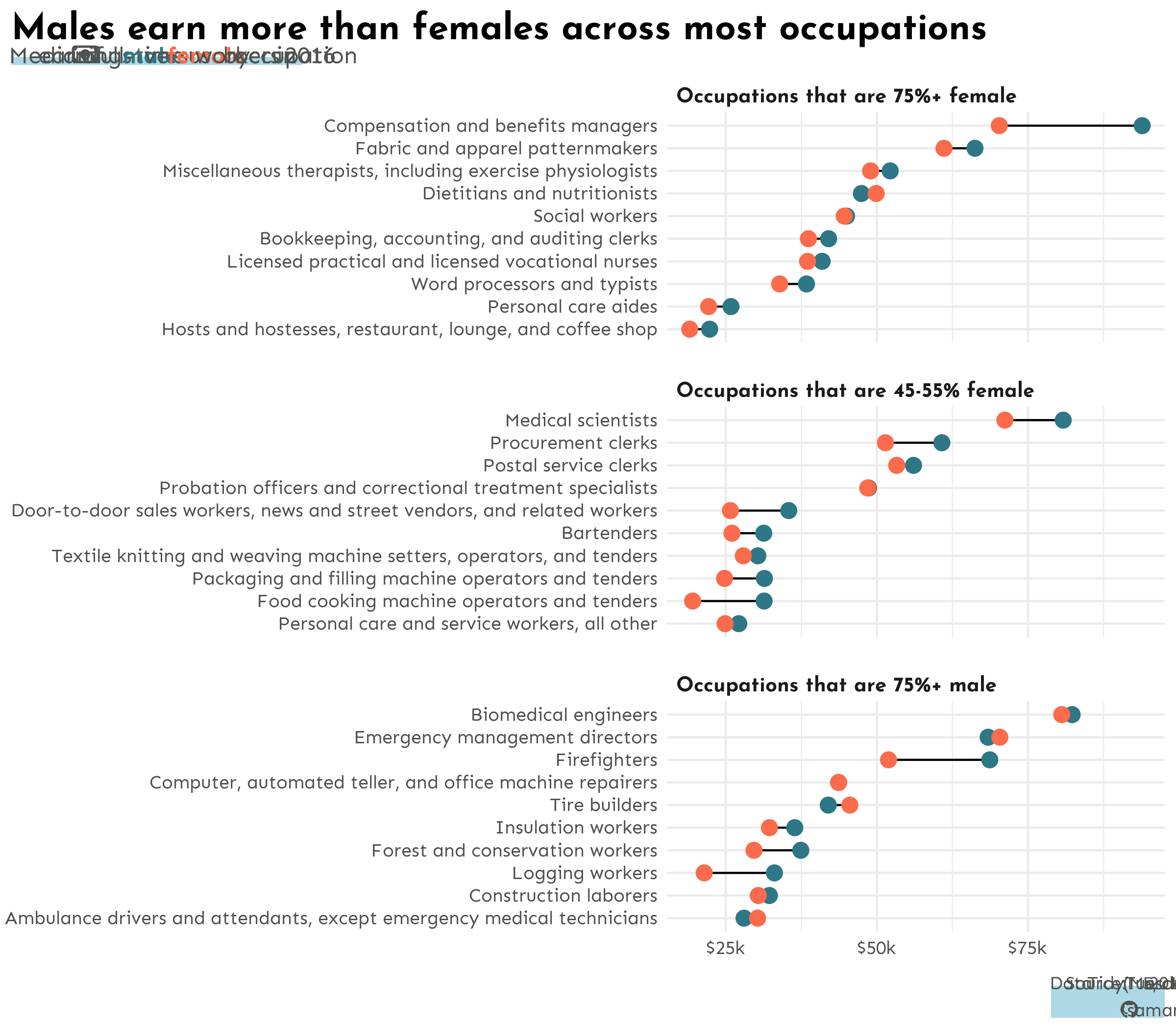
Our text wraps onto itself because these element_textbox()es don’t scale to the size of our plot, when written to a PNG file.
Let’s try increasing our textbox width
updated_plot <- plot +
  labs(title = "Males earn more than females across most occupations",
       subtitle = subtitle,
       caption = caption) +
  theme_minimal() +
  theme(
    plot.title.position = "plot",
    plot.title = element_text(family = "josefin",
                              face = "bold",
                              size = 18),
    plot.subtitle = ggtext::element_textbox(family = "sen",
                                            size = 12,
                                            color = earnings_pal["light_text"],
                                            fill = "lightblue", # for debugging
                                            width = unit(25, "cm"),
                                            margin = margin(t = 2, r = 0, b = 6, l = 0)),
    plot.caption = ggtext::element_textbox(family = "sen",
                                           face = "italic", # NOTE: this no longer applies since the typeface "sen" does not exist in an italic font style
                                           color = earnings_pal["light_text"],
                                           fill = "lightblue", # for debugging
                                           halign = 1,
                                           lineheight = 1.5,
                                           width = unit(25, "cm"),
                                           margin = margin(t = 15, r = 0, b = 0, l = 0)),
    strip.text.x = element_text(family = "josefin",
                                face = "bold",
                                size = 10,
                                hjust = 0),
    panel.spacing.y = unit(0.5, "cm"),
    axis.text = element_text(family = "sen",
                             size = 9,
                             color = earnings_pal["light_text"]),
    axis.title = element_blank()
  )

updated_plot
We successfully increased the width of our two textboxes, but they appear quite narrow and our text still isn’t expanded correctly.
Next, let’s increase textbox padding
While margin sets the space around a textbox, padding sets the space around the text inside a textbox. Let’s increase the padding around the top and bottom of our subtitle and caption:
updated_plot <- plot +
  labs(title = "Males earn more than females across most occupations",
       subtitle = subtitle,
       caption = caption) +
  theme_minimal() +
  theme(
    plot.title.position = "plot",
    plot.title = element_text(family = "josefin",
                              face = "bold",
                              size = 18),
    plot.subtitle = ggtext::element_textbox(family = "sen",
                                            size = 12,
                                            color = earnings_pal["light_text"],
                                            fill = "lightblue", # for debugging
                                            width = unit(25, "cm"),
                                            margin = margin(t = 2, r = 0, b = 6, l = 0),
                                            padding = margin(t = 5, r = 0, b = 5, l = 0)),
    plot.caption = ggtext::element_textbox(family = "sen",
                                           face = "italic", # NOTE: this no longer applies since the typeface "sen" does not exist in an italic font style
                                           color = earnings_pal["light_text"],
                                           fill = "lightblue", # for debugging
                                           halign = 1,
                                           lineheight = 1.5,
                                           width = unit(25, "cm"),
                                           margin = margin(t = 15, r = 0, b = 0, l = 0),
                                           padding = margin(t = 10, r = 0, b = 10, l = 0)),
    strip.text.x = element_text(family = "josefin",
                                face = "bold",
                                size = 10,
                                hjust = 0),
    panel.spacing.y = unit(0.5, "cm"),
    axis.text = element_text(family = "sen",
                             size = 9,
                             color = earnings_pal["light_text"]),
    axis.title = element_blank()
  )

updated_plot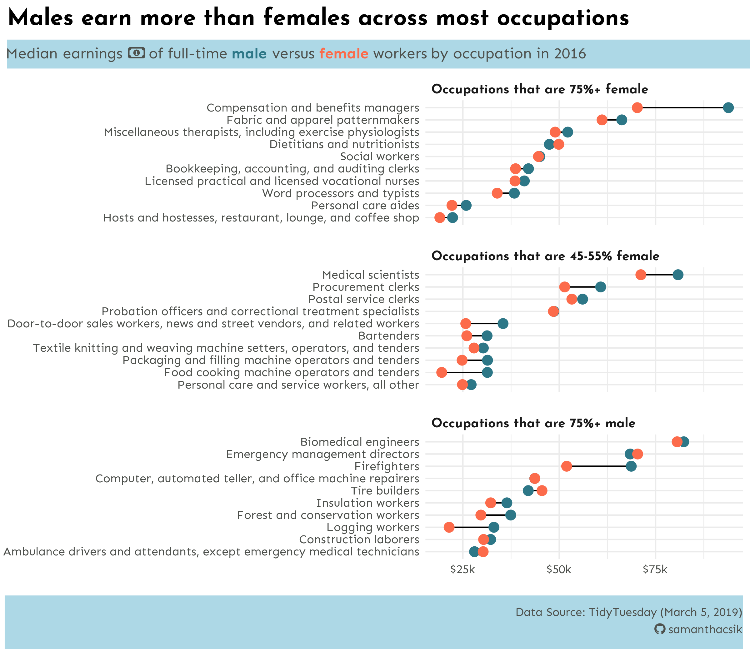
Yay! Looking good. We can now comment out (or remove) fill = "lightblue" from both our ggtext::element_textbox()es.
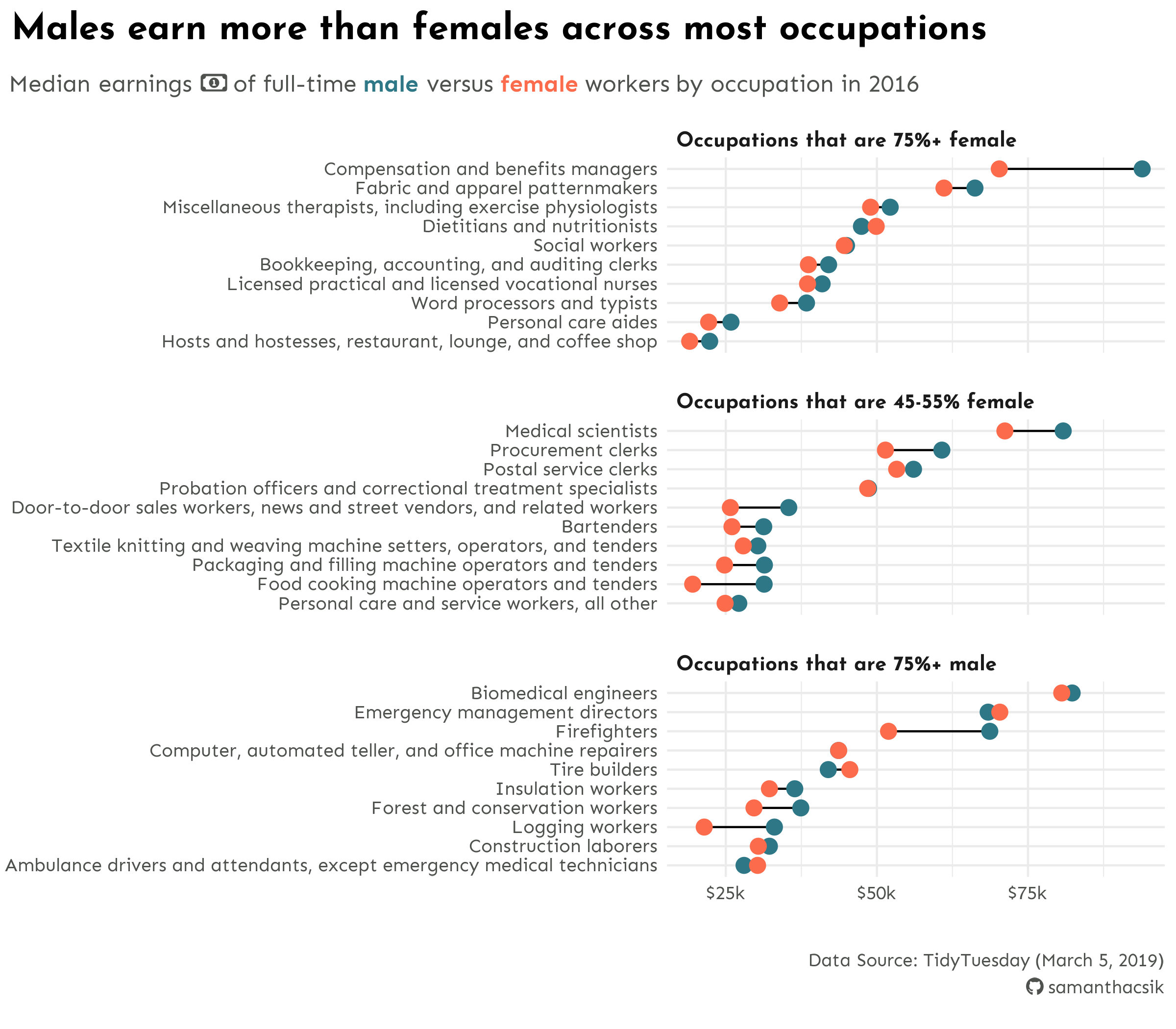
Our final saved PNG (8 x 7”, 300 DPI)!
Now let’s try saving a 14x12” plot
What happens?
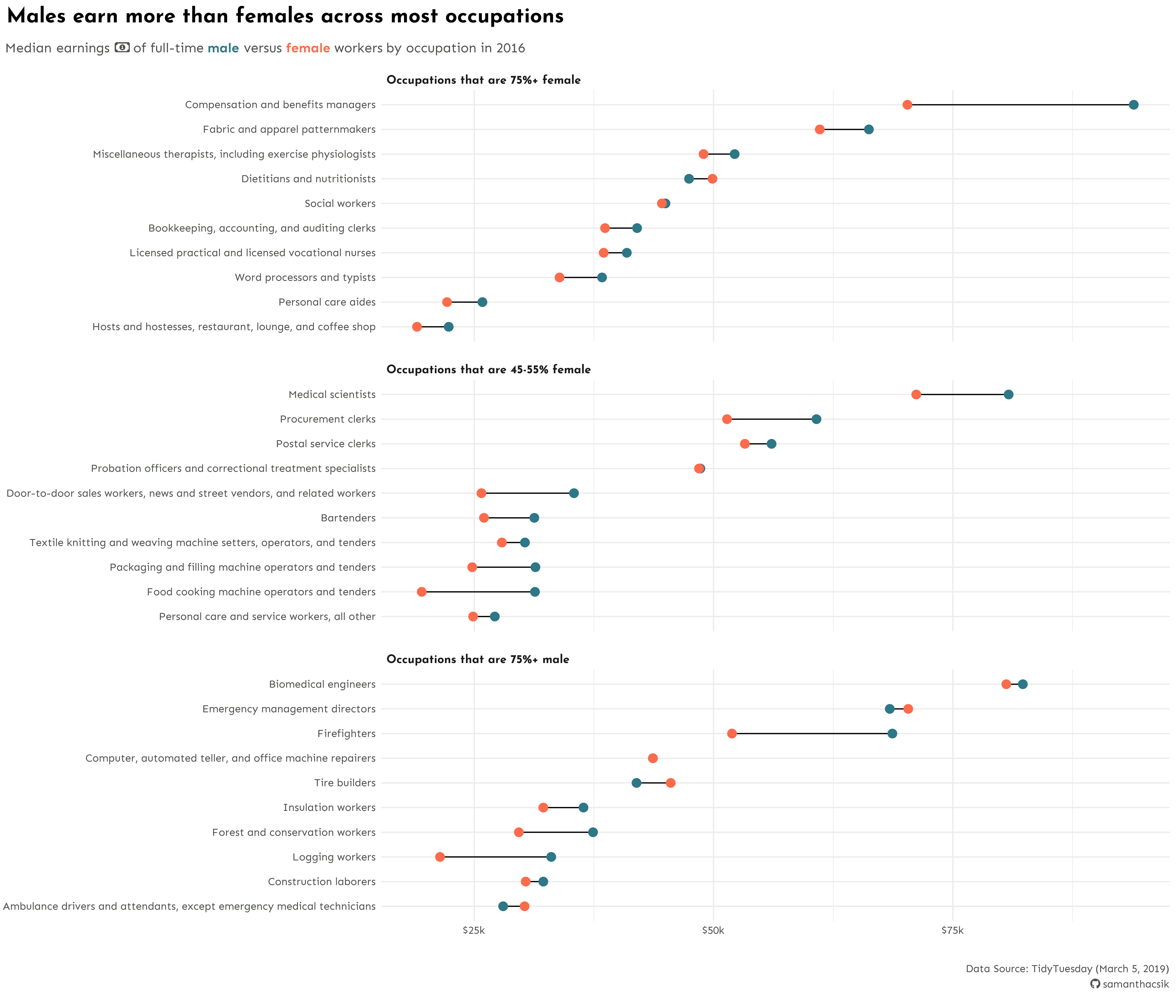
Our text shrunk again
We’ve set absolute text sizes
We’ve built our plot using absolute text sizes (where unit = “pt” = 0.33mm), which means our text sizes remain constant regardless of plot resizing (this is the case with any element defined in absolute units).
updated_plot <- plot +
  labs(title = "Males earn more than females across most occupations",
       subtitle = subtitle,
       caption = caption) +
  theme_minimal() +
  theme(
    plot.title.position = "plot",
    plot.title = element_text(family = "josefin",
                              face = "bold",
                              size = 18),
    plot.subtitle = ggtext::element_textbox(family = "sen",
                                            size = 12,
                                            color = earnings_pal["light_text"],
                                            # fill = "lightblue", # for debugging
                                            width = unit(25, "cm"),
                                            margin = margin(t = 2, r = 0, b = 6, l = 0),
                                            padding = margin(t = 5, r = 0, b = 5, l = 0)),
    plot.caption = ggtext::element_textbox(family = "sen",
                                           face = "italic", # NOTE: this no longer applies since the typeface "sen" does not exist in an italic font style
                                           color = earnings_pal["light_text"],
                                           # fill = "lightblue", # for debugging
                                           halign = 1,
                                           lineheight = 1.5,
                                           width = unit(25, "cm"),
                                           margin = margin(t = 15, r = 0, b = 0, l = 0),
                                           padding = margin(t = 10, r = 0, b = 10, l = 0)),
    strip.text.x = element_text(family = "josefin",
                                face = "bold",
                                size = 10,
                                hjust = 0),
    panel.spacing.y = unit(0.5, "cm"),
    axis.text = element_text(family = "sen",
                             size = 9,
                             color = earnings_pal["light_text"]),
    axis.title = element_blank()
  )

updated_plot
Instead, we can set relative text sizes
By setting size = rel(value), our text size will scale relative to the base_size, which by default is 11. We can also update the default base_size inside theme_minimal() (or whichever complete theme you’re using).
updated_plot <- plot +
  labs(title = "Males earn more than females across most occupations",
       subtitle = subtitle,
       caption = caption) +
  theme_minimal(base_size = 18) +
  theme(
    plot.title.position = "plot",
    plot.title = element_text(family = "josefin",
                              face = "bold",
                              size = rel(1.7)),
    plot.subtitle = ggtext::element_textbox(family = "sen",
                                            size = rel(1.1),
                                            color = earnings_pal["light_text"],
                                            # fill = "lightblue", # for debugging
                                            width = unit(25, "cm"),
                                            margin = margin(t = 2, r = 0, b = 6, l = 0),
                                            padding = margin(t = 5, r = 0, b = 5, l = 0)),
    plot.caption = ggtext::element_textbox(family = "sen",
                                           face = "italic", # NOTE: this no longer applies since the typeface "sen" does not exist in an italic font style
                                           color = earnings_pal["light_text"],
                                           # fill = "lightblue", # for debugging
                                           halign = 1,
                                           lineheight = 1.5,
                                           width = unit(25, "cm"),
                                           margin = margin(t = 15, r = 0, b = 0, l = 0),
                                           padding = margin(t = 10, r = 0, b = 10, l = 0)),
    strip.text.x = element_text(family = "josefin",
                                face = "bold",
                                size = rel(1.1),
                                hjust = 0),
    panel.spacing.y = unit(0.5, "cm"),
    axis.text = element_text(family = "sen",
                             size = rel(0.8),
                             color = earnings_pal["light_text"]),
    axis.title = element_blank()
  )

updated_plot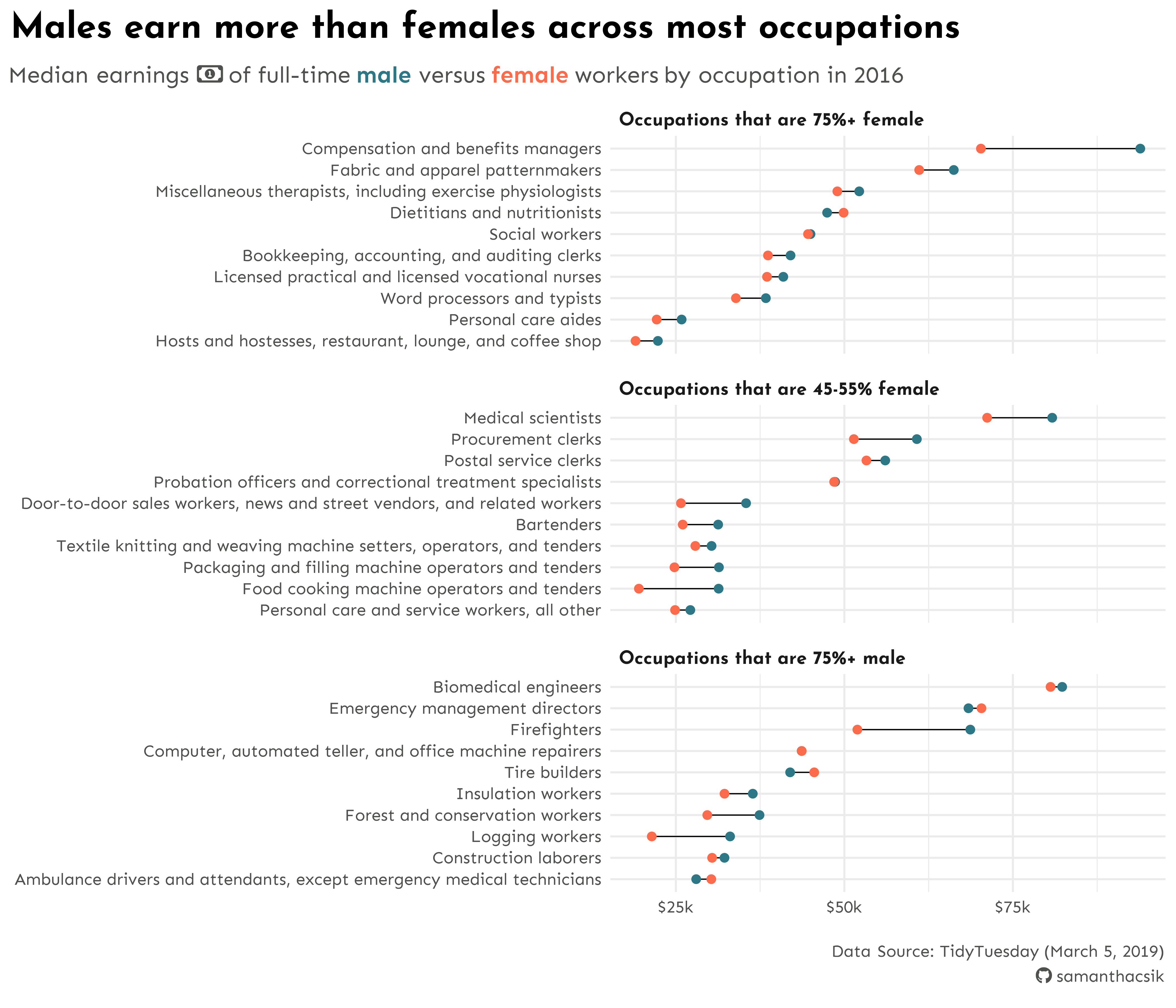
Our final saved PNG (14 x 12”, 300 DPI)!
One final exercise – save as 5x5” PNG
What happens?
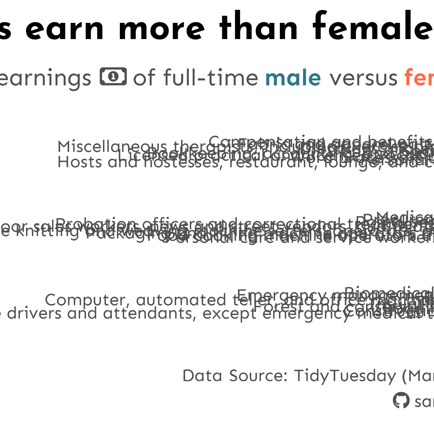
Noooo not again
Just adjust base_size!
This can take a little trial and error, but adjusting your text basesize (in this case, you’ll want to make it smaller) should do the trick – all relative text sizes will scale accordingly.
updated_plot <- plot +
  labs(title = "Males earn more than females across most occupations",
       subtitle = subtitle,
       caption = caption) +
  theme_minimal(base_size = 7) +
  theme(
    plot.title.position = "plot",
    plot.title = element_text(family = "josefin",
                              face = "bold",
                              size = rel(1.7)),
    plot.subtitle = ggtext::element_textbox(family = "sen",
                                            size = rel(1.1),
                                            color = earnings_pal["light_text"],
                                            # fill = "lightblue", # for debugging
                                            width = unit(25, "cm"),
                                            margin = margin(t = 2, r = 0, b = 6, l = 0),
                                            padding = margin(t = 5, r = 0, b = 5, l = 0)),
    plot.caption = ggtext::element_textbox(family = "sen",
                                           face = "italic", # NOTE: this no longer applies since the typeface "sen" does not exist in an italic font style
                                           color = earnings_pal["light_text"],
                                           # fill = "lightblue", # for debugging
                                           halign = 1,
                                           lineheight = 1.5,
                                           width = unit(25, "cm"),
                                           margin = margin(t = 15, r = 0, b = 0, l = 0),
                                           padding = margin(t = 10, r = 0, b = 10, l = 0)),
    strip.text.x = element_text(family = "josefin",
                                face = "bold",
                                size = rel(1.1),
                                hjust = 0),
    panel.spacing.y = unit(0.5, "cm"),
    axis.text = element_text(family = "sen",
                             size = rel(0.8),
                             color = earnings_pal["light_text"]),
    axis.title = element_blank()
  )

updated_plot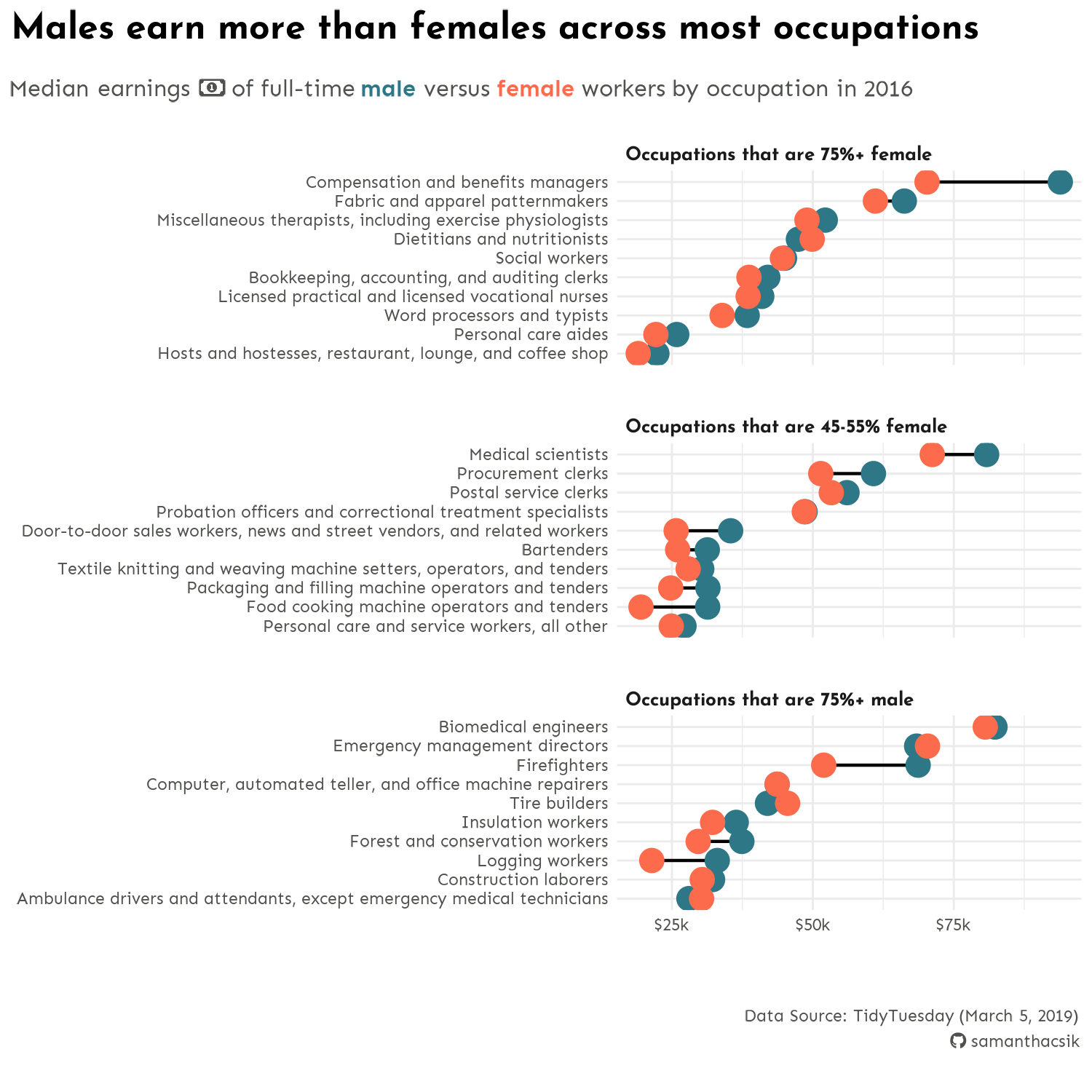
Note that we might consider adjusting our margins (e.g. between title and subtitle, between plot and caption), panel spacing, and point size which are defined in absolute units.
Margins use unit = "pt" = 0.35mm by default
To summarize:
- Make sure the resolution used by
{showtext}for text rendering matches the resolution used byggsave()for saving your plotshowtext_opts(dpi = 300)ggsave(dpi = 300)- 300 DPI is generally recommended
- Use relative text sizes wherever possible
- set a
base_sizein your complete theme - use
rel()to set relative text sizes
- set a
- Make absolute size adjustments as necessary
- e.g. to
{ggtext}elements, margins, panel spacing, point sizes, etc.
- e.g. to