Writing clean code

Writing clean, easily readable, and reproducible code is just as important as understanding any of the data visualization tools you’ll learn in this class. Now is the time to practice this skill so that you can take your beautiful code and styling skills with you into the workforce!

General conventions

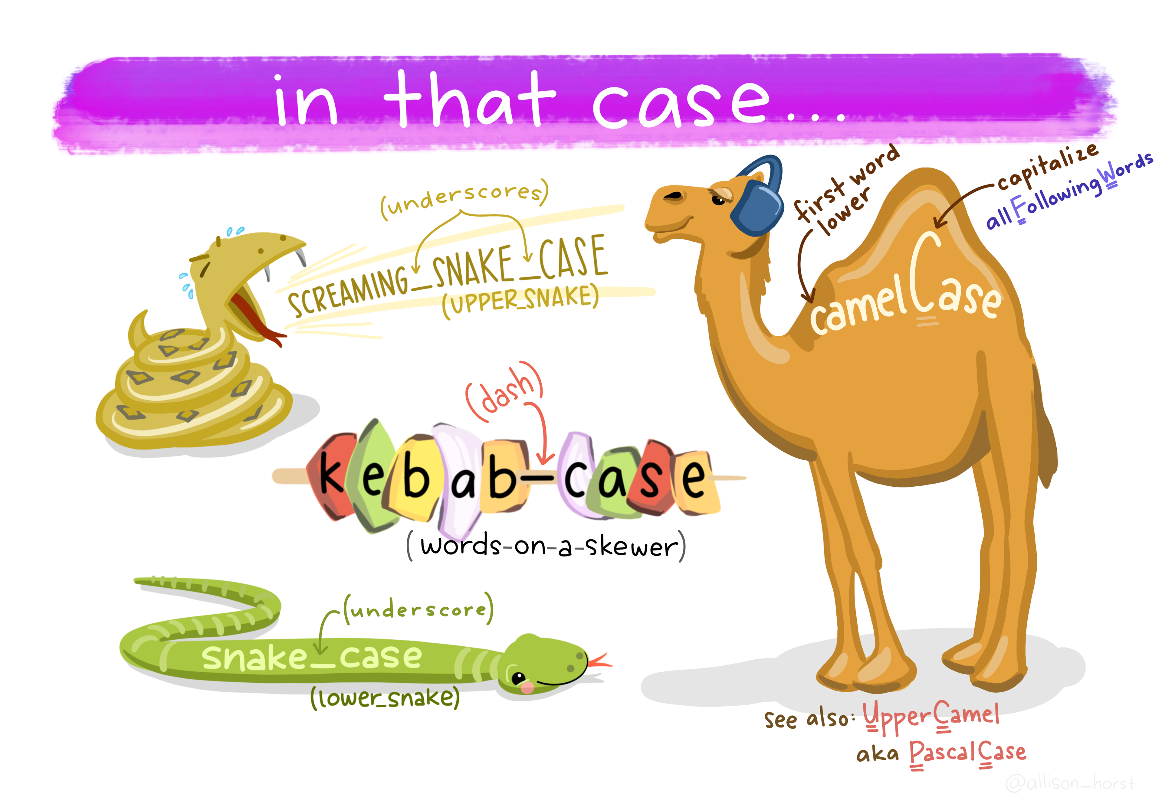
Stick to these standards (as suggested by The tidyverse style guide) whenever possible:

Naming conventions:

• Snake case for variable names – for example, my_data
• Kebab case for file names – for example, my-script.R

Art by Allison Horst

Whitespace conventions:

• Space around any infix operators (==, +, -, <-, etc) – for example:

my_data_clean <- my_data |> 
  filter(x == 2023)

• No space around operators with high precedence (::, :::, $, @, [, [[, ^, unary -, unary +, and :) – for example:

sqrt(x^2 + y^2)
df$z
x <- 1:10

• Space before a pipe, |> or %>%, and (most often) a new line after – for example:

my_data |> 
  filter(...)

• Space before a ggplot +, and a new line after – for example:

ggplot(data, aes(x = x, y = y)) +
  geom_point()

• Space between arguments, commas, and operators, but no space between a parentheses and the following or proceeding argument/value – for example:

ggplot(data, aes(x = x, y = y, color = z)) +
  geom_point(alpha = 0.8)

• Only one level of indentation when piping into a ggplot – for example:

data |> 
  filter(...) |> 
  ggplot(aes(x = x, y = y, fill = z)) +
  geom_point()

• If arguments to a ggplot layer don’t all fit on one line, put each argument on it’s own line and indent – for example:

ggplot(data, aes(x = x, y = y, color = z)) +
  geom_point() + 
  labs(
    x = "My x-axis label",
    y = "My y-axis label",
    title = "My plot title",
    caption = "My plot caption"
  )

Annotating code

The {ARTofR} package is wonderful for creating clean titles, dividers, and block comments for your code. Install the RStudio Addin, or call {ARTofR} functions in your console to generate comments, copy to your clipboard, and paste into your scripts.

I’ve always opted for the console approach:

1. Load the package (library(ARTofR)) in your console (rather than in your script / qmd file)
2. Type your preferred divider (see the package README for options) and message, also in the console
3. The resulting divider is automatically copied to your clipboard
4. Paste into your script

A couple dividers that I use often:

• For major section dividers, xxx_title2("text here") renders as:

##~~~~~~~~~~~~~~~~~~~~~~~~~~~~~~~~~~~~~~~~~~~~~~~~~~~~~~~~~~~~~~~~~~~~~~~~~~~~~~
##                                  text here                               ----
##~~~~~~~~~~~~~~~~~~~~~~~~~~~~~~~~~~~~~~~~~~~~~~~~~~~~~~~~~~~~~~~~~~~~~~~~~~~~~~

• For subsection dividers, xxx_divider1("text here") renders as:

#............................text here...........................

• For line-level annotations, I also often use (not created using {ARTofR}):

# text here ---- 

Here’s a short example script demonstrating how I like to use these dividers:

##~~~~~~~~~~~~~~~~~~~~~~~~~~~~~~~~~~~~~~~~~~~~~~~~~~~~~~~~~~~~~~~~~~~~~~~~~~~~~~
##                                    Setup                                 ----
##~~~~~~~~~~~~~~~~~~~~~~~~~~~~~~~~~~~~~~~~~~~~~~~~~~~~~~~~~~~~~~~~~~~~~~~~~~~~~~

#.........................load libraries.........................
library(tidyverse)
library(palmerpenguins)

#..........................import data...........................
# ~ if you're reading in data, this is a great place to do it ~
  
##~~~~~~~~~~~~~~~~~~~~~~~~~~~~~~~~~~~~~~~~~~~~~~~~~~~~~~~~~~~~~~~~~~~~~~~~~~~~~~
##                          Data wrangling / cleaning                       ----
##~~~~~~~~~~~~~~~~~~~~~~~~~~~~~~~~~~~~~~~~~~~~~~~~~~~~~~~~~~~~~~~~~~~~~~~~~~~~~~

penguins_wrangled <- penguins |> 
  
  # select relevant cols ----
  select(species, bill_length_mm, bill_depth_mm, year) |> 
  
  # filter for year of interest ----
  filter(year == 2009)

##~~~~~~~~~~~~~~~~~~~~~~~~~~~~~~~~~~~~~~~~~~~~~~~~~~~~~~~~~~~~~~~~~~~~~~~~~~~~~~
##                             Data visualization                           ----
##~~~~~~~~~~~~~~~~~~~~~~~~~~~~~~~~~~~~~~~~~~~~~~~~~~~~~~~~~~~~~~~~~~~~~~~~~~~~~~

# histogram of penguin bill lengths in the year 2009 ----
ggplot(penguins, aes(x = bill_length_m, fill = species)) +
  geom_histogram()

# scatterplot of penguin bill lengths by bill depths in the year 2009 ----
ggplot(penguins_wrangled, aes(x = bill_length_mm, y = bill_depth_mm, color = species)) +
  geom_point()

Style guides

• Tidyverse style guide, by Hadley Wickham – a book that describes the style used throughout the {tidyverse}
• Tidy design principles, by Hadley Wickham – a book to help you write better R code (currently under development)