Fundamental chart types (evolution & amounts / rankings)

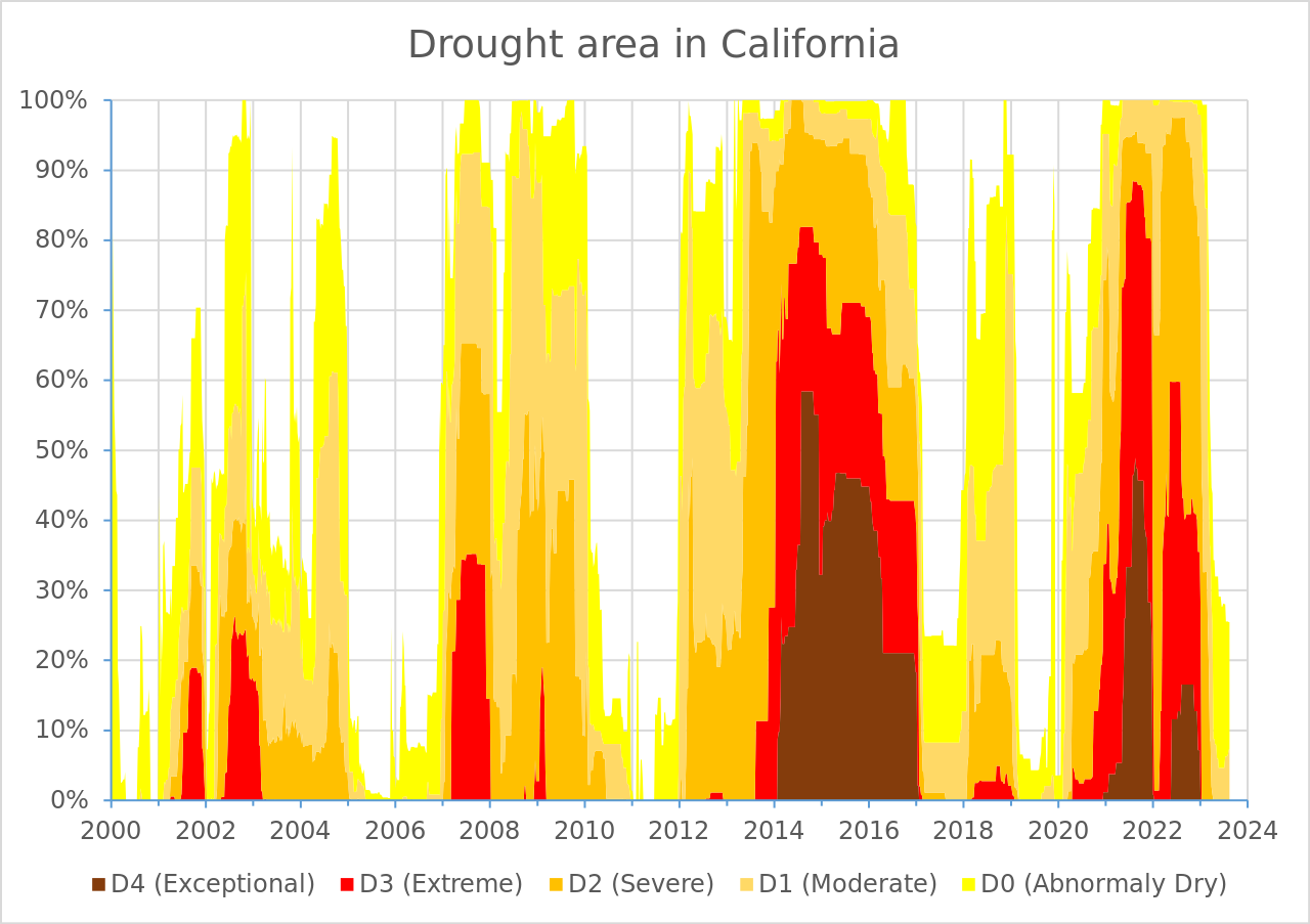
U.S. Drought Monitor’s California assessment. Source: Wikipedia. We’ll talk about stacked area charts in this week’s lecture and you’ll recreate this viz during lab session.

Pre-class Prep

A. Install required packages

install.packages("usethis") # for editing .Renviron (see step C. in pre-class prep)
install.packages("tidytuesdayR") # used to download TidyTuesday data
install.packages("tidycensus") # an R package that allows users to interface with a select number of the US Census Bureau’s data APIs and return tidyverse-ready data frames
install.packages("scales") # provides the internal scaling infrastructure used by ggplot2, and gives you tools to override the default breaks, labels, transformations and palettes (installed automatically with {ggplot2} or {tidyverse})

B. Download data

Save data to your class repo at EDS-240-class-examples/week3/data/:

Lecture	Dataset title	Download link	Notes
3.1	USGS National Water Availability Assessment Outputs (CONUS 2025)	download the combined IWA .csv file from the National Water Availability Assessment Data Companion (NWDC) (Google Drive backup link, in case the NWDC is unavailable)	These data are modeled estimates of monthly water supply and use (not empirical measurements from sensors / gauges); Read more about the model & data
3.2	Lyme Disease Cases by State or Locality	download link (Google Drive backup link, in case CDC portal is unavailable)	Data made available by the CDC (read more on the CDC’s Lyme Disease Surveillance Data page; see other available data under Dashboard data files)
3.2	US Census Bureau Population Estimates Program	we’ll use the {tidycensus} package to interface with the US Census Bureau’s API and download the data programmatically (see step C, below, for setup instructions), however, in the event that the API is down, you can access a backup copy of the 2019 vintage on Google Drive	Read more about The Census Bureau’s Population Estimates Program (PEP)

C. Request a US Census Bureau API key & add it to your .Renviron file

1. To use the {tidycensus} package to access US Census Bureau data, you’ll first need to request and activate an API key. Do so by following these steps:

   1. Request an API key at http://api.census.gov/data/key_signup.html
   2. After a short period of time, you should receive an email with your key (it may be helpful to star / bookmark that email), and click the included link to activate your key (Note: if you get an error when activating your key, close your browser window and try clicking the activation link again).

2. Add your API key to your .Renviron file. For security purposes, you should NEVER push any API keys to GitHub. Rather than typing our API key into any of our scripts, we can instead save it to and read it from our .Renviron file. Follow these steps:

   1. Run usethis::edit_r_environ() in your Console, which will open up your .Renviron file (it will create it if you don’t already have one).
   2. Store envrionment variables as key / value pairs. Add your API key as shown, below, then save and restart R for your changes to take effect.

.Renviron

# be sure to name it exactly as written here (all caps) 
CENSUS_API_KEY="XXXXXXXXXXXXXXXXXXXXXXXXXXXXXXXXXXXXXXXX"

• Note: You may also consider storing your API key in a password manager for safe keeping (e.g. in case your computer decides to call a quits, is lost, etc.)

What exactly is .Renviron?

Dotfiles (files which are preceded by a dot, .) are hidden files, which are broadly used to customize the behavior of programs. You may already be familiar with some dotfiles, such as .gitconfig and .gitignore.

The .Renviron file is an R-specific dotfile, which is commonly used for (though not limited to) storing sensitive information, such as API keys. It lives in your computer’s home directory (e.g. /Users/yourUserName on macOS, or C:/Users/yourUserName/Documents on Windows), and is automatically sourced when an R session starts. When sourced, all stored variables (such as your API key) are made available to your R environment for you to use. Variables should be stored as key / value pairs (e.g. KEY_NAME="VALUE". Access them using Sys.getenv("KEY_NAME").

Oftentimes, packages that are built to interface with APIs will include their own helper functions for adding API keys to your .Renviron file (e.g. see tidycensus::census_api_key()). You may choose to use these helper functions in place of usethis::edit_r_environ(), if you prefer.

D. Download .qmd templates & review initial data wrangling code

1. Download all necessary templates (links in the table below) and save them to a EDS-240-data-viz-examples/week3/ folder.

2. Review the data wrangling code under the ## Setup section of each template file and make note of any questions you might have. Due to time constraints, we won’t be live-coding our way through the data wrangling code in class. However, we’ll reserve some time to answer any questions before we jump into data viz .

Lecture Materials

Lecture slides	Code-along template	Code-along key
Lecture 3.1: visualizing amounts / rankings	3.1 template	3.1 key
Lecture 3.2: visualizing evolution	3.2 template	3.2 key

Pre-lab Prep

A. Download data

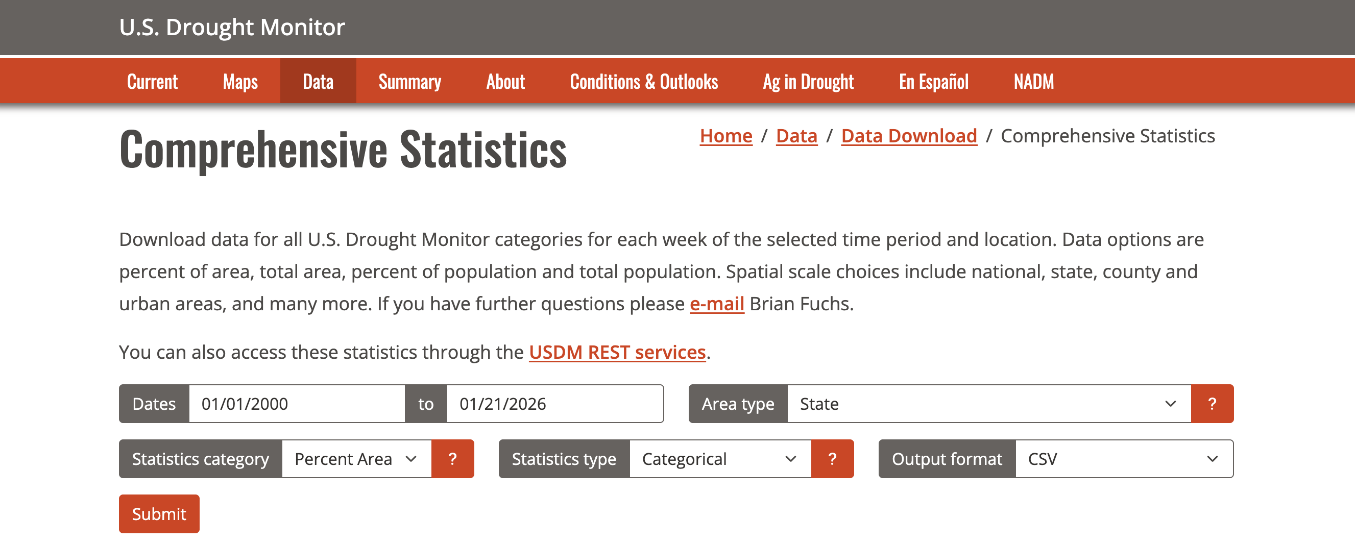
Head to the Comprehensive Statistics Download Data page on the USDM Website. Select the following options, click “Submit”, and save the downloaded data to your class repo at EDS-240-class-examples/week3/data/

Dataset title	Download link	Notes
US Drought Monitor Comprehensive Statistics	download the .csv file that is generated with the above specifications from the Comprehensive Statistics Data Download Page on the USDM Website (Google Drive backup link, in case the USDM is unavailable)	NA

B. Prepare a week3-lab.qmd file

Add a new blank file to your class repo at the following location: EDS-240-class-examples/week3/week3-lab.qmd. Fill out the necessary YAML information (title, author, date + any other information you find helpful).

C. (OPTIONAL) Install Chrome extension for picking colors

Install the ColorZilla Google Chrome extension (also available for Firefox), which makes it easy to select color values from webpages.

Lab Materials

Lab Slides	Exercise instructions	Exercise solutions
Lab 3 slides: USDM	Lab 3 exercise: recreate USDM viz	Lab 3 solution

Assignment Reminders

Assignment Type	Assignment Title	Date Assigned	Date Due
FPM	Final Project Milestone #1	Wed 01/07/2026	Wed 01/21/2026, 11:59pm PT
HW	Homework #2	Wed 01/21/2026	Wed 01/28/2026, 11:59pm PT