##~~~~~~~~~~~~~~~~~~~~~~~~~~~~~~~~~~~~~~~~~~~~~~~~~~~~~~~~~~~~~~~~~~~~~~~~~~~~~~
## setup ----
##~~~~~~~~~~~~~~~~~~~~~~~~~~~~~~~~~~~~~~~~~~~~~~~~~~~~~~~~~~~~~~~~~~~~~~~~~~~~~~
#..........................load packages.........................
library(tidyverse)
#..........................import data...........................
# data preprocessing
drought <- read_csv(here::here("week3", "data", "drought.csv"))
##~~~~~~~~~~~~~~~~~~~~~~~~~~~~~~~~~~~~~~~~~~~~~~~~~~~~~~~~~~~~~~~~~~~~~~~~~~~~~~
## wrangle drought data ----
##~~~~~~~~~~~~~~~~~~~~~~~~~~~~~~~~~~~~~~~~~~~~~~~~~~~~~~~~~~~~~~~~~~~~~~~~~~~~~~
drought_clean <- drought |>
# Pivot table to be in tidy form
pivot_longer(cols = None:D4, names_to = "drought_lvl", values_to = "area_pct") |>
janitor::clean_names() |>
# Rename state abbreviation column
rename(state_abb = state_abbreviation) |>
# select cols of interest & update names for clarity (as needed) ----
select(date = valid_start, state_abb, drought_lvl, area_pct) |>
# add year, month & day cols using {lubridate} fxns ----
# NOTE: this step isn't necessary for our plot, but I'm including as examples of how to extract different date elements from a object of class Date using {lubridate} ----
mutate(year = year(date),
month = month(date, label = TRUE, abbr = TRUE),
day = day(date)) |>
# add drought level conditions names ----
mutate(drought_lvl_long = factor(drought_lvl,
levels = c("D4", "D3", "D2", "D1","D0", "None"),
labels = c("D4 (Exceptional)", "(D3) Extreme",
"D2 (Severe)", "D1 (Moderate)",
"D0 (Abnormaly Dry)",
"No Drought"))) |>
# reorder cols ----
relocate(date, year, month, day, state_abb, drought_lvl, drought_lvl_long, area_pct)
##~~~~~~~~~~~~~~~~~~~~~~~~~~~~~~~~~~~~~~~~~~~~~~~~~~~~~~~~~~~~~~~~~~~~~~~~~~~~~~
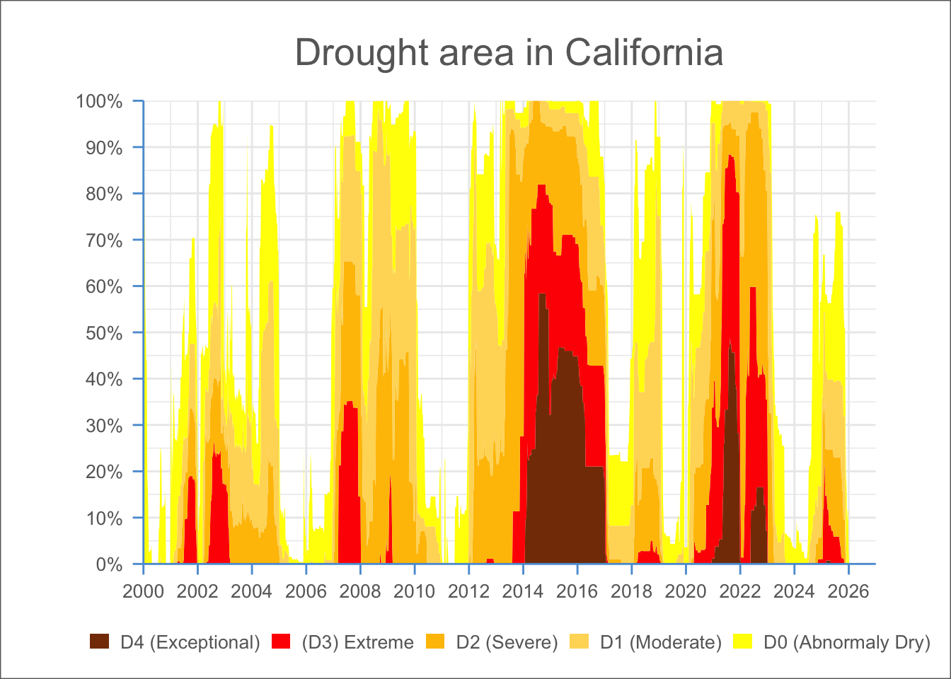
## create stacked area plot of CA drought conditions through time ----
##~~~~~~~~~~~~~~~~~~~~~~~~~~~~~~~~~~~~~~~~~~~~~~~~~~~~~~~~~~~~~~~~~~~~~~~~~~~~~~
drought_clean |>
# remove drought_lvl "None" & filter for just CA ----
filter(drought_lvl != "None",
state_abb == "CA") |>
# initialize ggplot ----
ggplot(mapping = aes(x = date, y = area_pct, fill = drought_lvl_long)) +
# reverse order of groups so level D4 is closest to x-axis ----
geom_area(position = position_stack(reverse = TRUE)) +
# update colors to match US Drought Monitor ----
# (colors identified using ColorPick Eyedropper extension on the original USDM data viz)
scale_fill_manual(values = c("#853904", "#FF0000", "#FFC100", "#FFD965", "#FFFF00")) +
# set x-axis breaks & remove padding between data and x-axis ----
scale_x_date(breaks = scales::breaks_pretty(n = 13),
limits = as.Date(c("2000-01-01", "2026-12-31")),
expand = c(0,0)) +
# set y-axis breaks & remove padding between data and y-axis & convert values to percentages ----
scale_y_continuous(breaks = seq(0, 100, by = 10),
expand = c(0, 0),
labels = scales::label_percent(scale = 1)) +
# add title ----
labs(title = "Drought area in California") +
##~~~~~~~~~~~~~~~~~~~~~~~~~~~~~~~~~~~~~~~~~~~~~~~~~~~~~~~~~~~~~~~~~~~~~~~~~~~~~~
## --
##------------------------- THEME CODE!-----------------------------
## --
##~~~~~~~~~~~~~~~~~~~~~~~~~~~~~~~~~~~~~~~~~~~~~~~~~~~~~~~~~~~~~~~~~~~~~~~~~~~~~~
# set theme minimal (includes major/minor grid lines, no axes) ----
theme_minimal() +
# fine-tune adjustments to plot theme ----
theme(
# update axis lines & ticks color ----
axis.line = element_line(color = "#5A9CD6"),
axis.ticks = element_line(color = "#5A9CD6"),
# adjust length of axis ticks ----
axis.ticks.length = unit(.2, "cm"),
# center plot title ----
plot.title = element_text(hjust = 0.5, color = "#686868", size = 20,
margin = margin(t = 10, r = 0, b = 15, l = 0)),
# remove axis & legend titles ----
axis.title = element_blank(),
legend.title = element_blank(),
# axis text color & size ----
axis.text = element_text(color = "#686868", size = 10),
legend.text = element_text(color = "#686868", size = 10),
# move legend below plot ----
legend.position = "bottom",
legend.direction = "horizontal",
legend.key.width = unit(0.4, "cm"),
legend.key.height = unit(0.25, "cm"),
plot.background = element_rect(color = "#686868"),
plot.margin = margin(t = 10, r = 40, b = 10, l = 40)
)