This template follows lecture 5.2 slides. Please be sure to cross-reference the slides, which contain important information and additional context!
Setup
##~~~~~~~~~~~~~~~~~~~~~~~~~~~~~~~~~~~~~~~~~~~~~~~~~~~~~~~~~~~~~~~~~~~~~~~~~~~~~~
## setup ----
##~~~~~~~~~~~~~~~~~~~~~~~~~~~~~~~~~~~~~~~~~~~~~~~~~~~~~~~~~~~~~~~~~~~~~~~~~~~~~~
#..........................load packages.........................
library(palmerpenguins)
library(tidyverse)
##~~~~~~~~~~~~~~~~~~~~~~~~~~~~~~~~~~~~~~~~~~~~~~~~~~~~~~~~~~~~~~~~~~~~~~~~~~~~~~
## create base plots ----
##~~~~~~~~~~~~~~~~~~~~~~~~~~~~~~~~~~~~~~~~~~~~~~~~~~~~~~~~~~~~~~~~~~~~~~~~~~~~~~
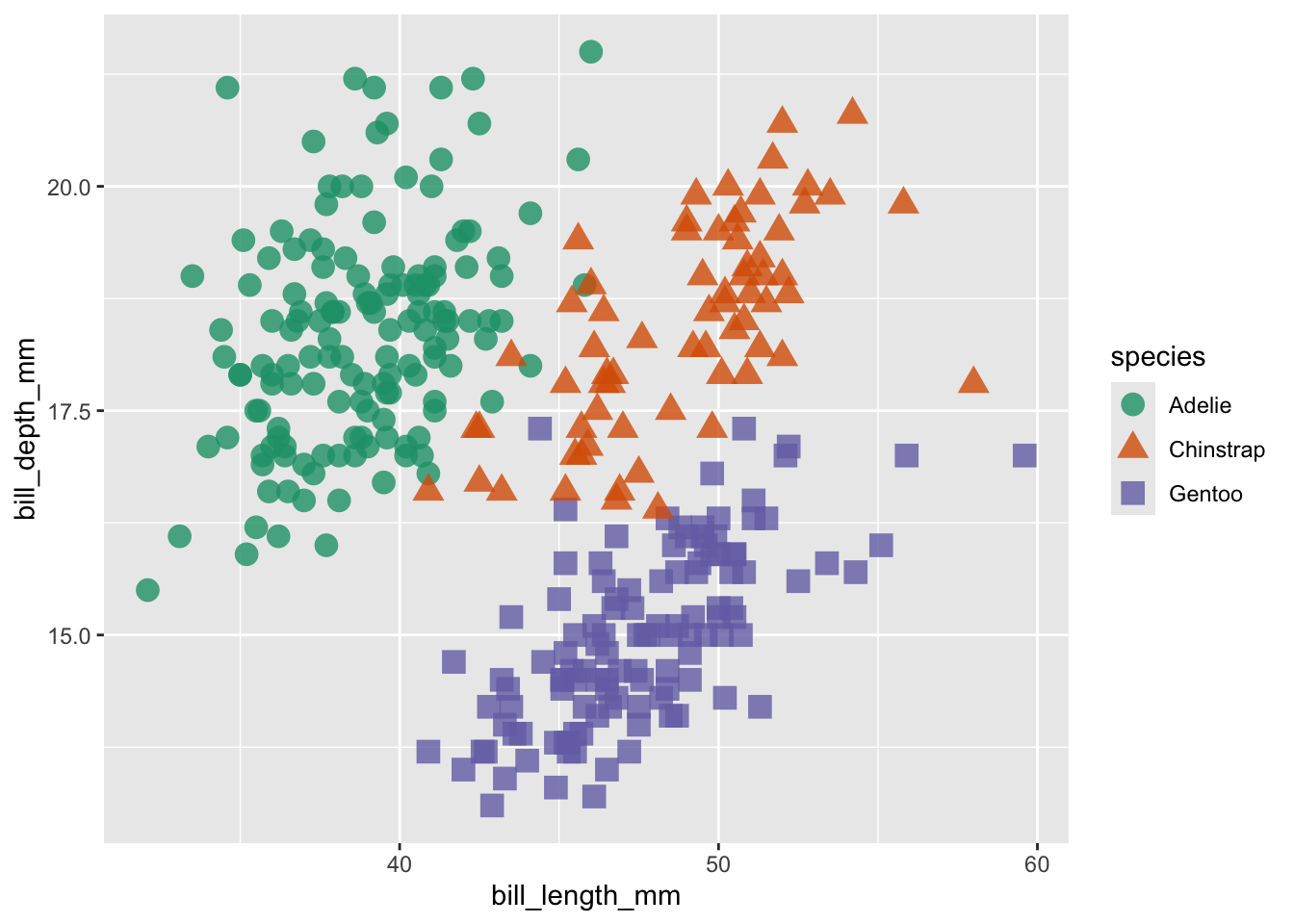
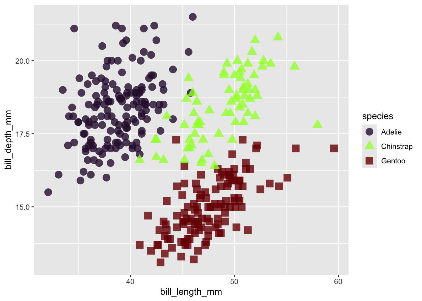
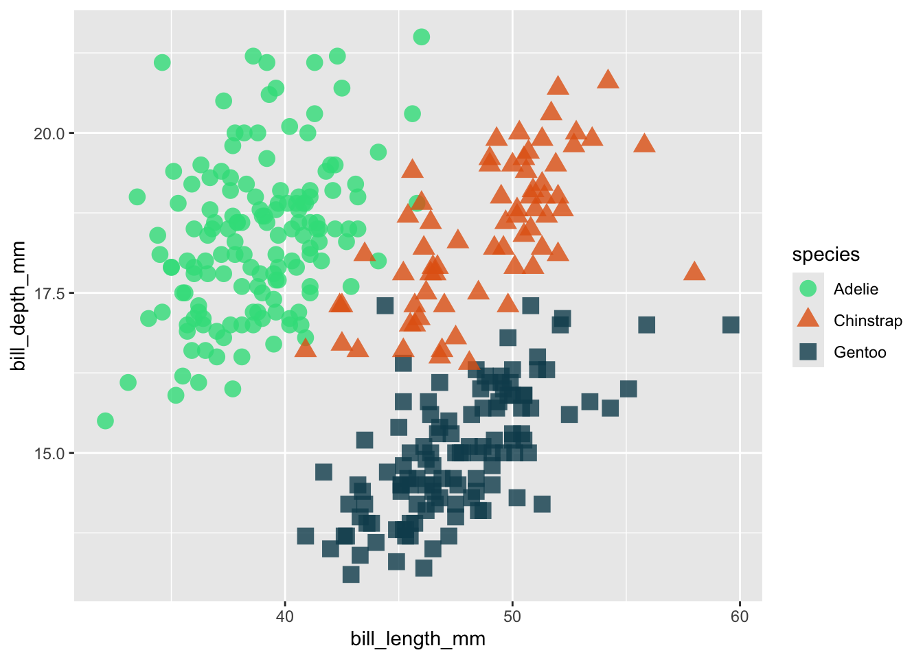
# requires categorical color scale ----
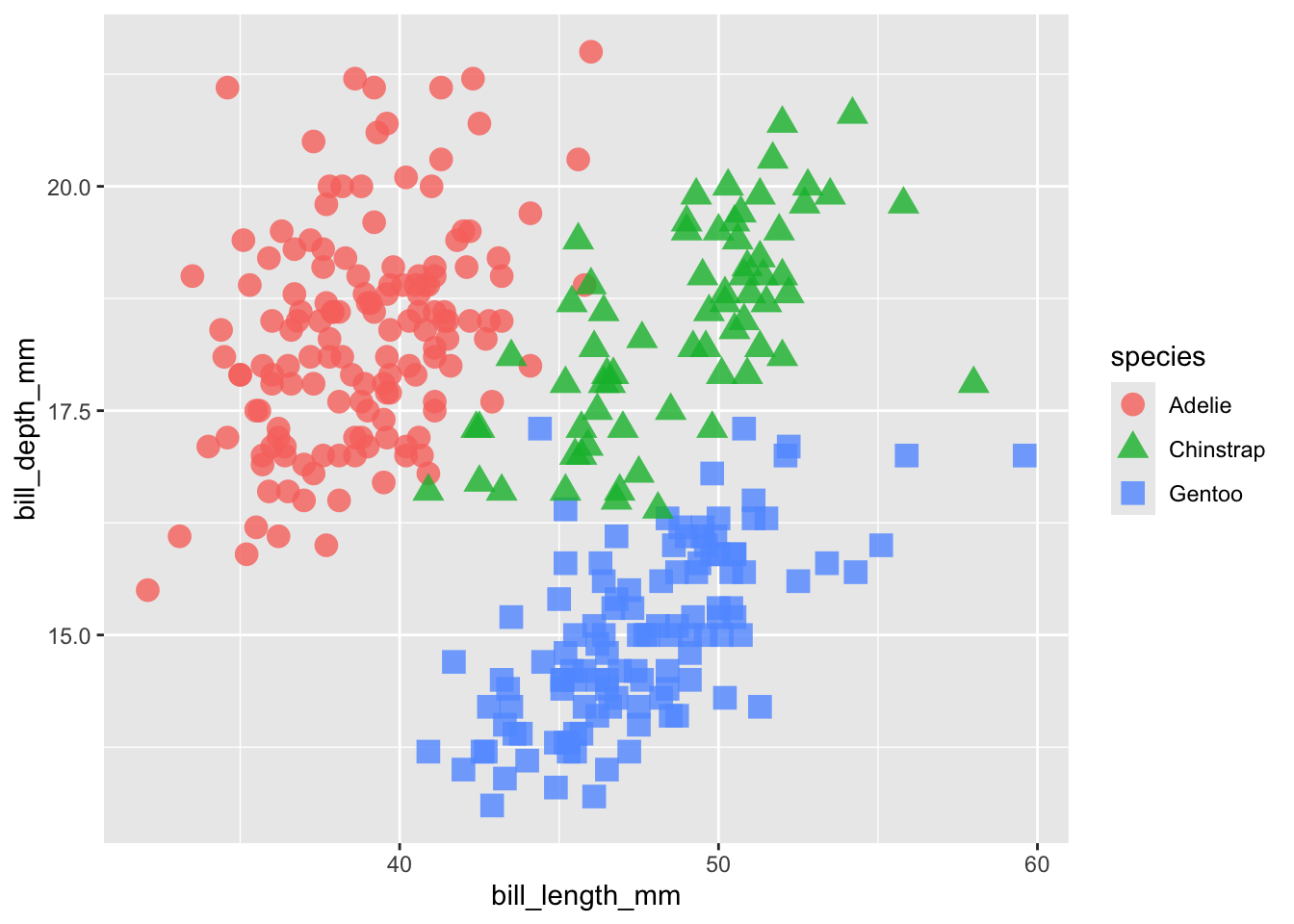
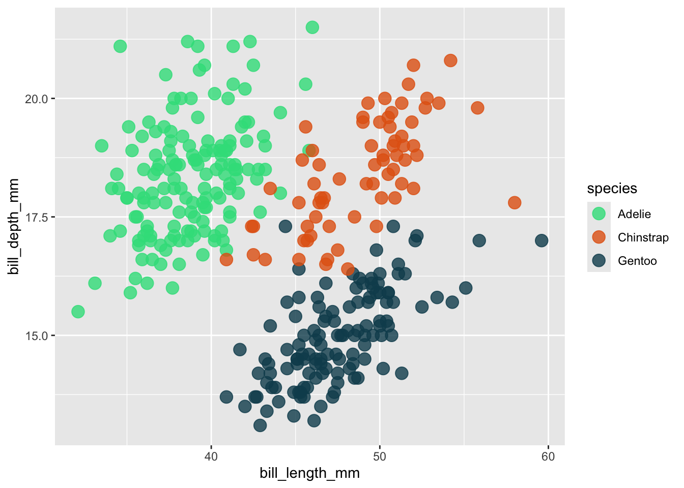
cat_color_plot <- ggplot(na.omit(penguins),
aes(x = bill_length_mm, y = bill_depth_mm,
color = species, shape = species)) +
geom_point(size = 4, alpha = 0.8)
cat_color_plot
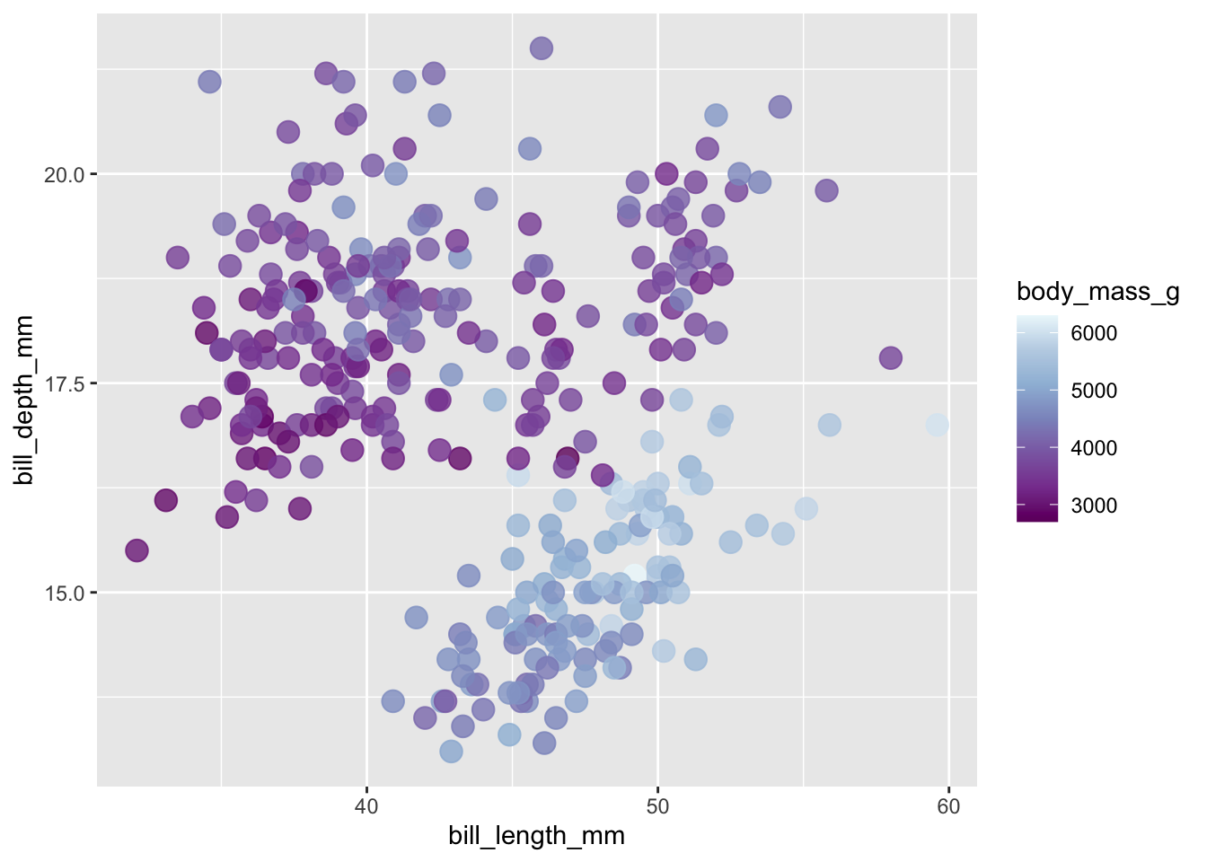
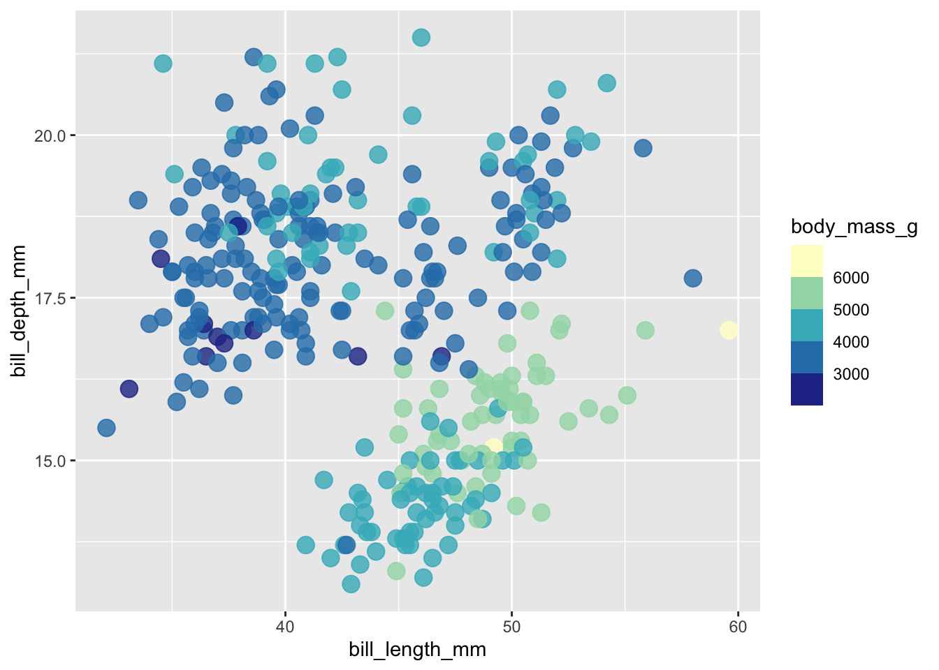
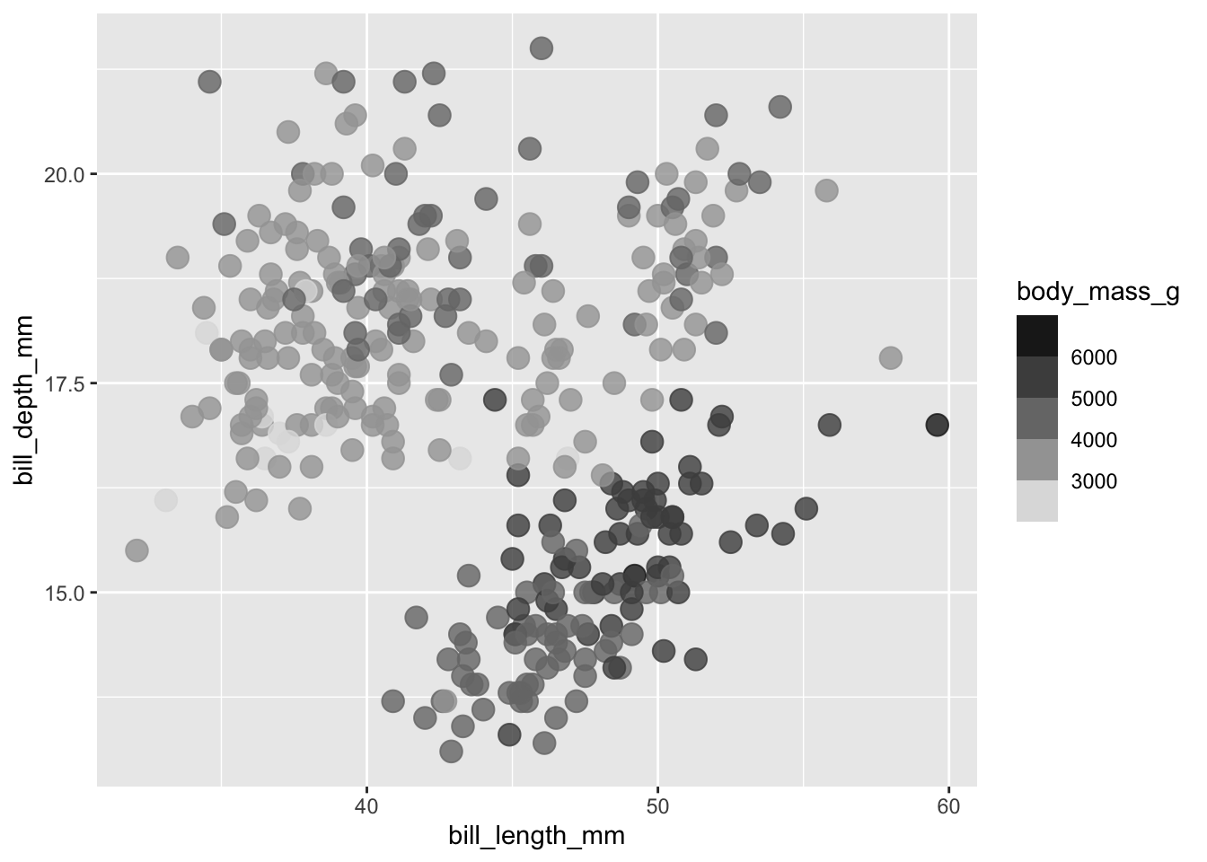
# requires continuous color scale ----
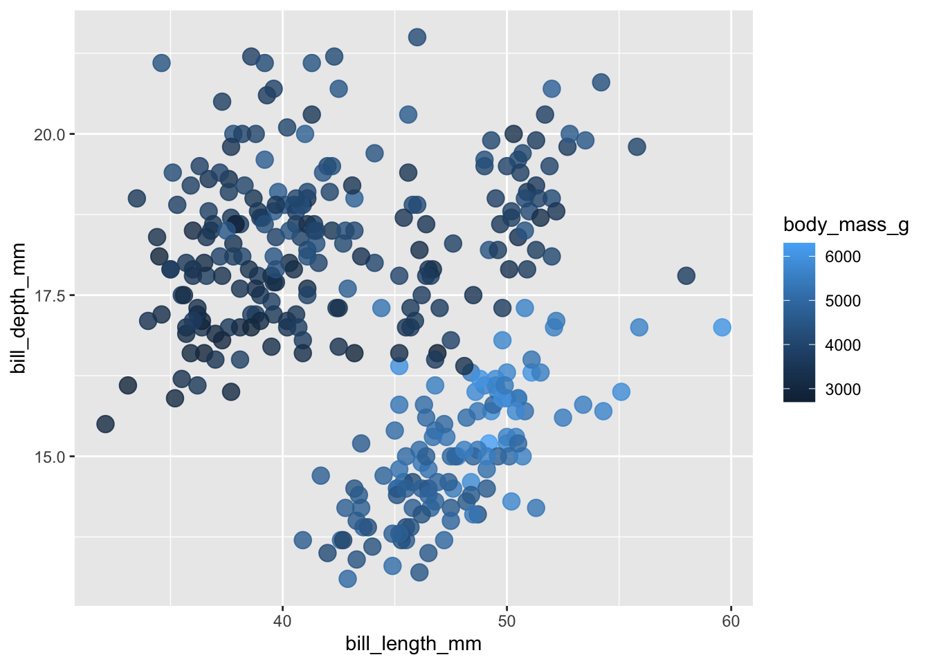
con_color_plot <- ggplot(na.omit(penguins),
aes(x = bill_length_mm, y = bill_depth_mm,
color = body_mass_g)) +
geom_point(size = 4, alpha = 0.8)
con_color_plot
Colors for inclusive & accessible design
Viridis scales
- Check out the documentation for additional viridis palette options.
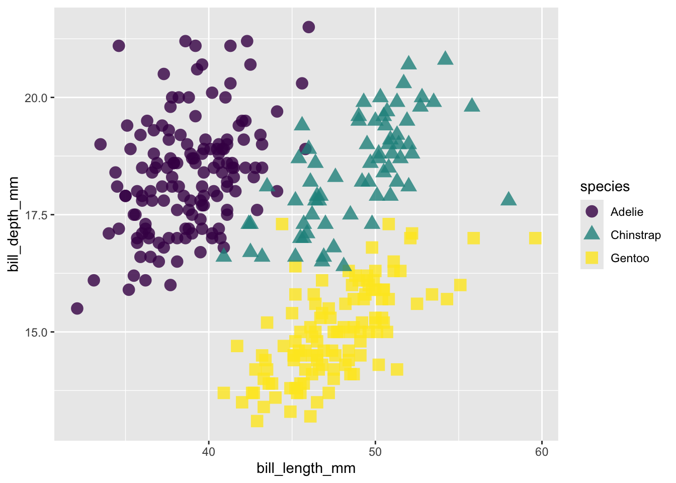
# discrete viridis scales ----
cat_color_plot +
  scale_color_viridis_d(option = "viridis")
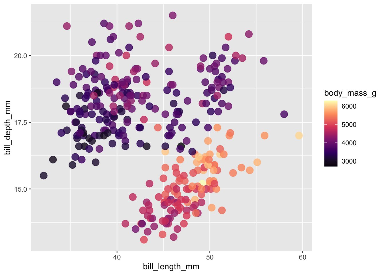
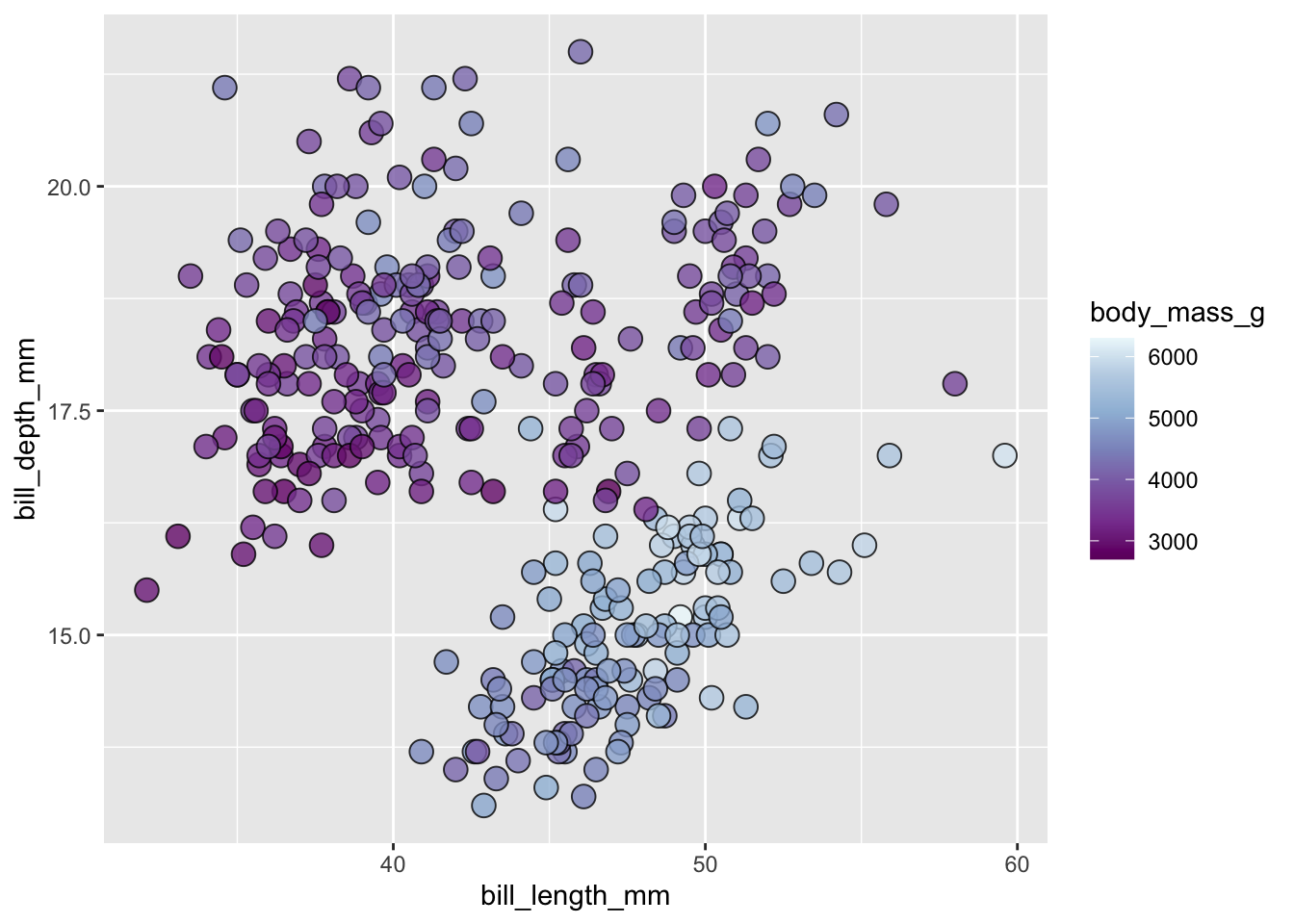
# continuous color scales ----
con_color_plot +
  scale_color_viridis_c(option = "magma")
RColorBrewer scales
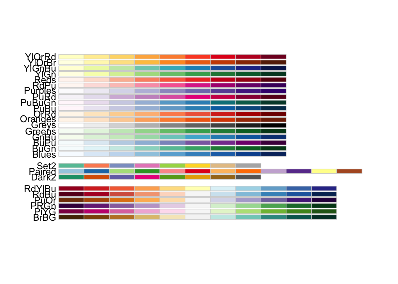
# display only colorblind-friendly RColorBrewer palettes ----
RColorBrewer::display.brewer.all(colorblindFriendly = TRUE)
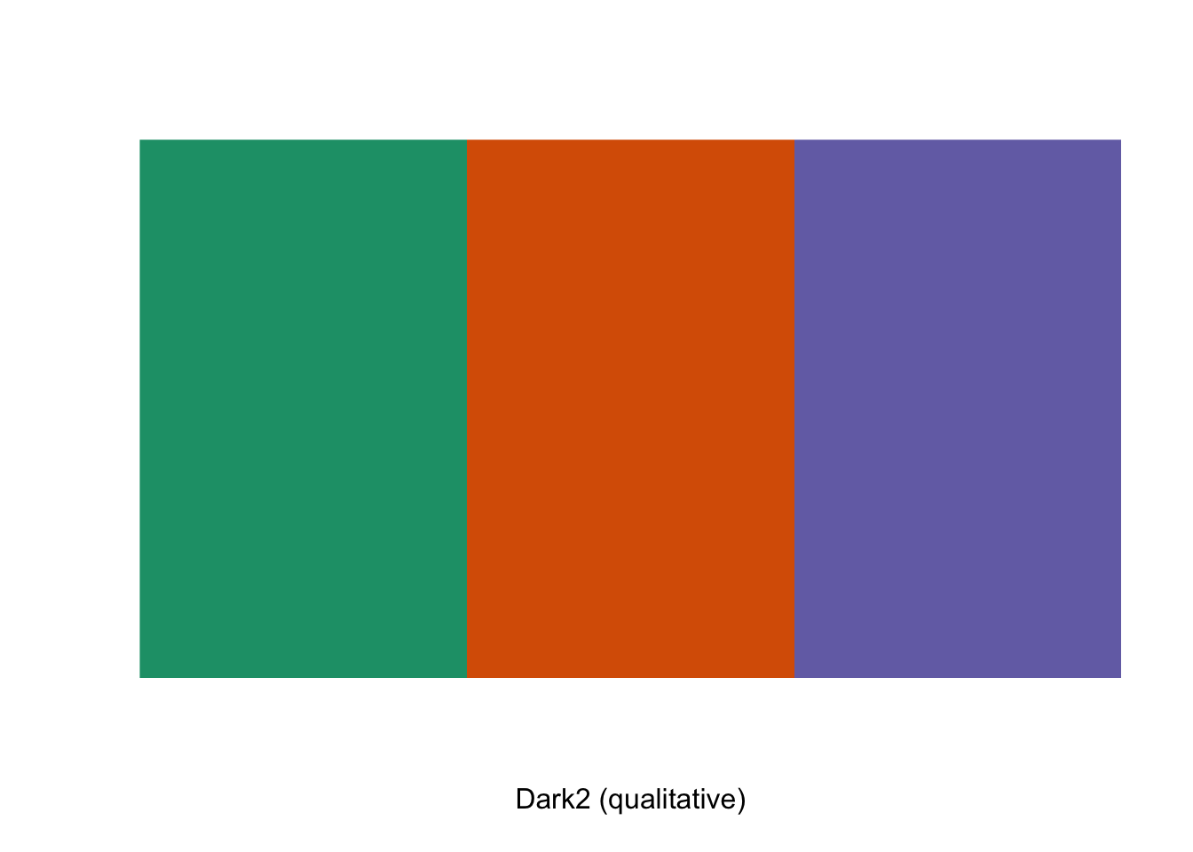
# preview palette with your number of desired colors ----
RColorBrewer::display.brewer.pal(n = 3, name = "Dark2")
# print the HEX codes of your palette ----
RColorBrewer::brewer.pal(n = 3, name = "Dark2")
[1] "#1B9E77" "#D95F02" "#7570B3"
# or save hex codes as a vector ----
my_brewer_pal <- RColorBrewer::brewer.pal(n = 3, name = "Dark2")
- Using RColorBrewer palettes
# for qualitative palettes ----
cat_color_plot +
  scale_color_brewer(palette = "Dark2")
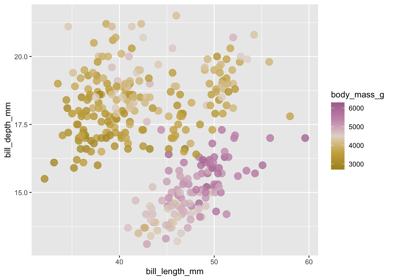
# for unclassed continuous color scales ----
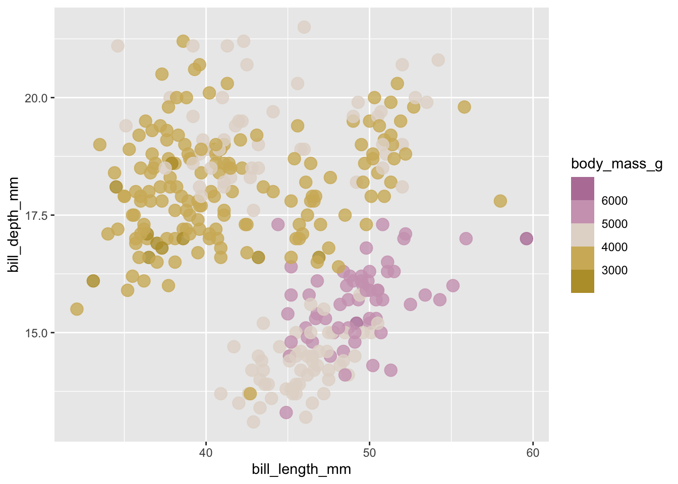
con_color_plot +
scale_color_distiller(palette = "BuPu")
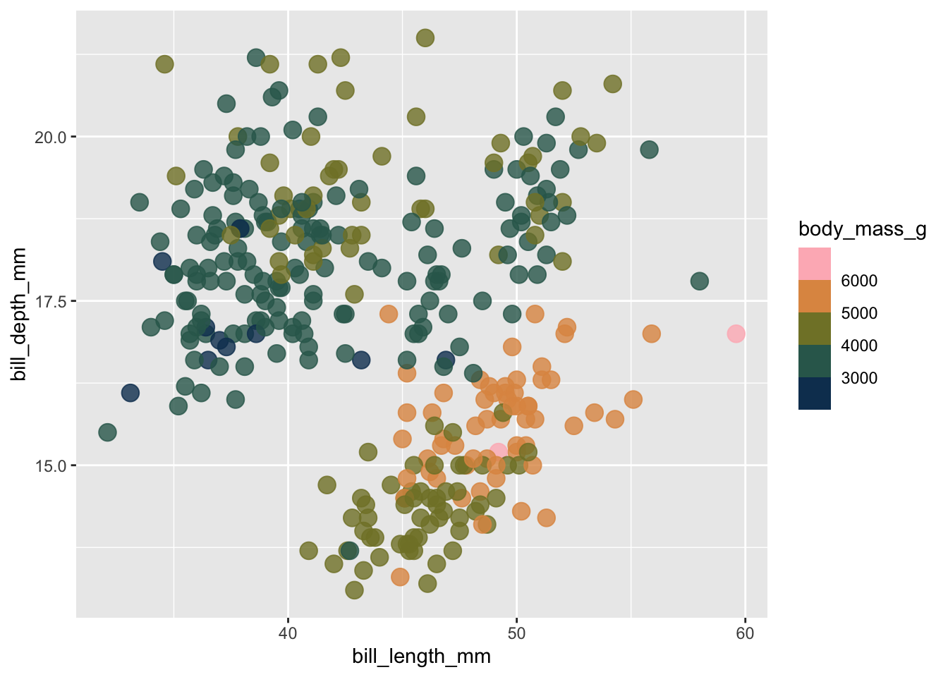
# for classed continuous color scales ----
con_color_plot +
  scale_color_fermenter(palette = "YlGnBu")
Accessibility tips
- outline light-colored points, which are difficult to see
ggplot(penguins, aes(x = bill_length_mm, y = bill_depth_mm, fill = body_mass_g)) +
  geom_point(shape = 21, size = 4, alpha = 0.8) +
  scale_fill_distiller(palette = "BuPu")
- use redundant mapping (colors & shapes) whenever possible
ggplot(penguins, aes(x = bill_length_mm, y = bill_depth_mm, color = species, shape = species)) +
  geom_point(size = 4, alpha = 0.8) +
  scale_color_viridis_d(option = "turbo")
Paletteer
# import {paletteer} ----
library(paletteer)
Explore available packages in the form of built-in data frames:
# view names of supported pkgs/palettes ----
View(palettes_d_names)
View(palettes_c_names)
I. apply palette using scale_*_paletteer_*()
# discrete data / palette ----
cat_color_plot +
  paletteer::scale_color_paletteer_d("calecopal::superbloom3")
# continuous data / palette (unclassed) ----
con_color_plot +
  paletteer::scale_color_paletteer_c("scico::batlow", direction = -1)
# continuous data / palette (classed) ----
con_color_plot +
  paletteer::scale_color_paletteer_binned("scico::batlow")
II. create vector of colors using paletteer_*(), then apply using the appropriate ggplot::scale_*() function
- discrete data / palette example:
# view names of pkgs/palettes ----
# View(palettes_d_names)

# create palette ----
pal_d <- paletteer::paletteer_d("wesanderson::GrandBudapest1", n = 3)
pal_d
<colors>
#F1BB7BFF #FD6467FF #5B1A18FF
# apply to scatter plot (use `color` variant) ----
cat_color_plot +
  scale_color_manual(values = pal_d)
# apply to histogram (use `fill` variant) ----
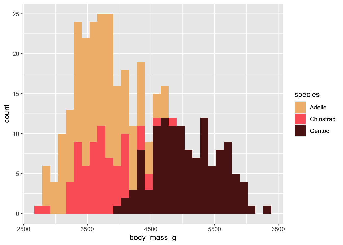
ggplot(penguins, aes(x = body_mass_g, fill = species)) +
geom_histogram() +
scale_fill_manual(values = pal_d)
- continuous data / palette example:
# view names of pkgs/palettes ----
# View(palettes_c_names)

# create palette ----
pal_c <- paletteer::paletteer_c("scico::grayC", n = 5, direction = -1)
pal_c
<colors>
#FFFFFFFF #AFAFAFFF #777777FF #434343FF #000000FF
# apply to scatter plot as an unclassed palette (use `gradientn` variant) ----
con_color_plot +
  scale_color_gradientn(colors = pal_c)
# apply to scatter plot as a classed (binned) palette (use `stepsn` variant) ----
con_color_plot +
  scale_color_stepsn(colors = pal_c)
Subduing pure hues
- Adjust saturation when selecting a HEX code from Google’s color picker, https://g.co/kgs/9SQkdgv, or adjust chroma directly in your ggplot:
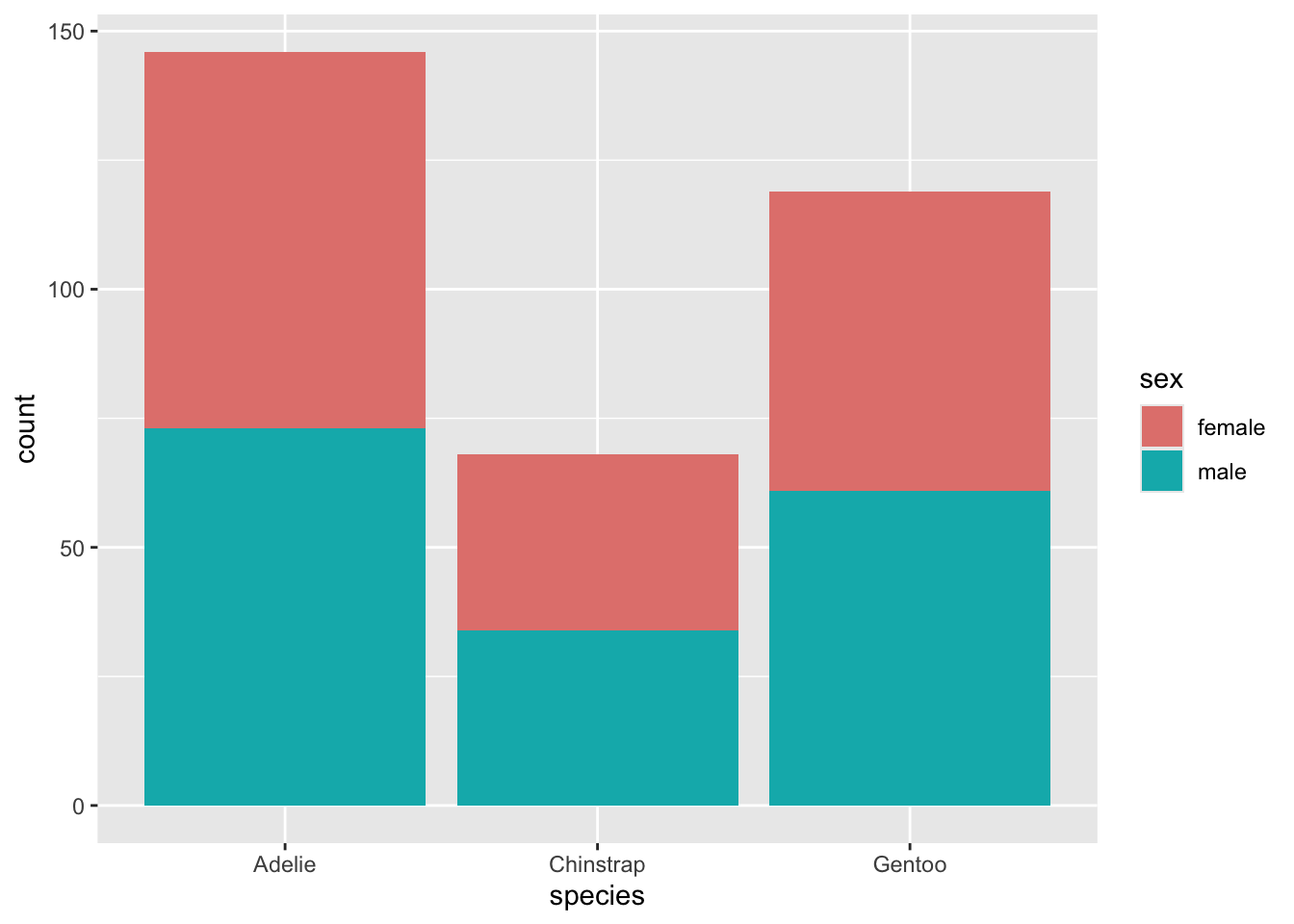
ggplot(na.omit(penguins), aes(x = species, fill = sex)) +
  geom_bar() +
  scale_fill_hue(c = 70)
- Adjust value when selecting a HEX code from Google’s color picker, https://g.co/kgs/9SQkdgv, or adjust lightness directly in your ggplot:
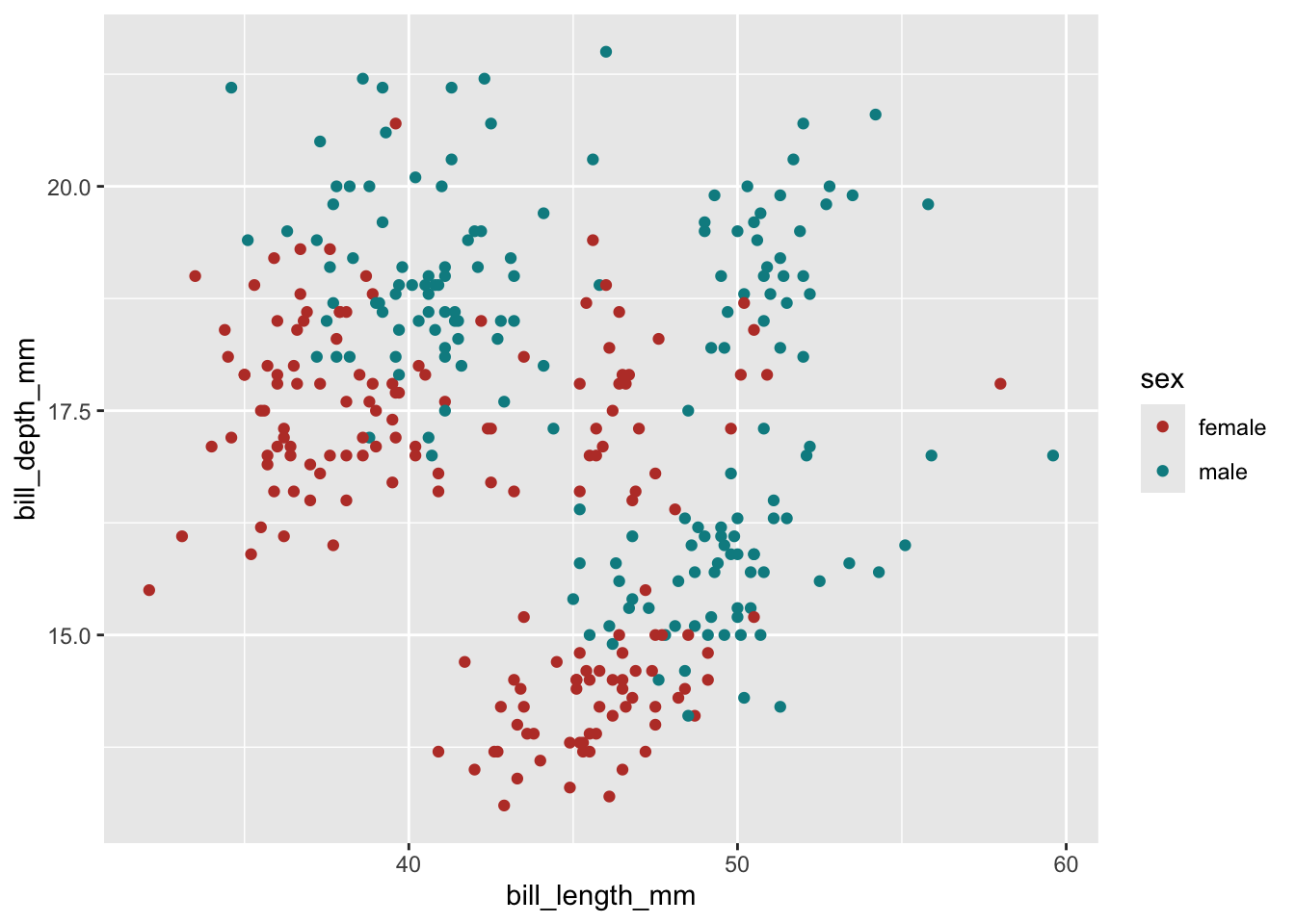
ggplot(na.omit(penguins), aes(x = bill_length_mm, y = bill_depth_mm, color = sex)) +
  geom_point() +
  scale_color_hue(l = 45)
- Increase transparency using the
alpha argument in ggplot
ggplot(penguins, aes(x = species)) +
  geom_bar(fill = "#00FF33", color = "gray7", alpha = 0.5) +
  theme_classic()
Some final palette tips
Save palette outside of plot
# create palette ----
my_palette <- c("#32DE8A", "#E36414", "#0F4C5C")

# apply to plot ----
cat_color_plot +
  scale_color_manual(values = my_palette)
Set color names
# create palette ----
my_palette_named <- c("Adelie" = "#32DE8A","Chinstrap" = "#E36414", "Gentoo" = "#0F4C5C")

# apply to plot (all penguins) ----
ggplot(penguins, aes(x = bill_length_mm, y = bill_depth_mm, color = species)) +
  geom_point(size = 4, alpha = 0.8) +
  scale_color_manual(values = my_palette_named)
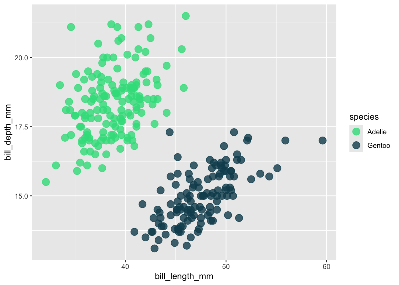
# apply to plot (just adelie & gentoo) ----
penguins |>
  filter(species != "Chinstrap") |>
  ggplot(aes(x = bill_length_mm, y = bill_depth_mm, color = species)) +
  geom_point(size = 4, alpha = 0.8) +
  scale_color_manual(values = my_palette_named)
Use scale_*_identity()
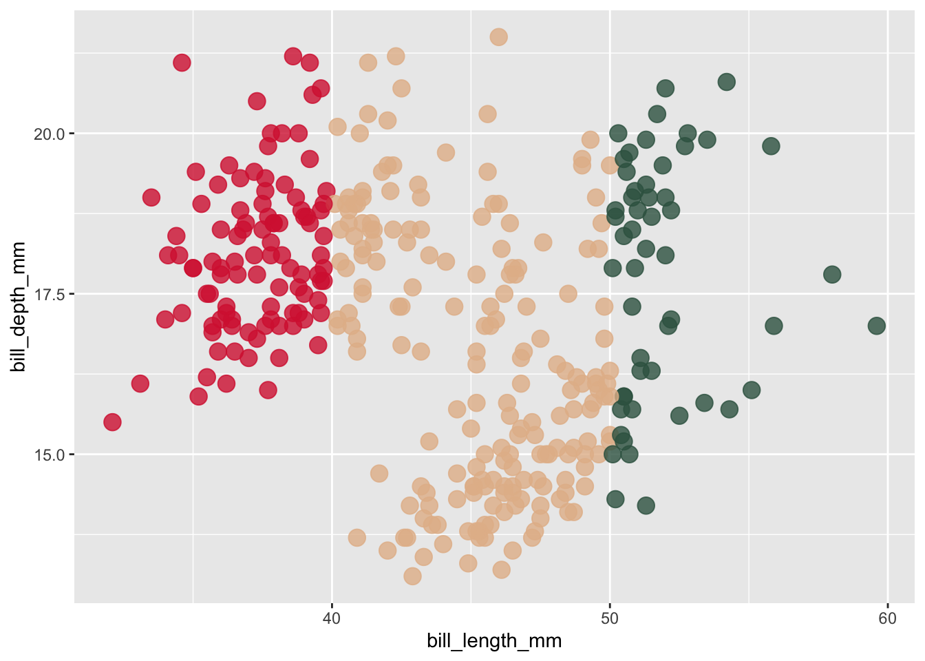
- Ex 1: color points based on value
# example 1 ----
penguins_ex1 <- penguins |>
  mutate(
    my_color = case_when(
      bill_length_mm < 40 ~ "#D7263D",
      between(x = bill_length_mm, left = 40, right = 50) ~ "#E4BB97",
      bill_length_mm > 50 ~ "#386150"
    )
  )

ggplot(penguins_ex1, aes(x = bill_length_mm, y = bill_depth_mm, color = my_color)) +
  geom_point(size = 4, alpha = 0.8) +
  scale_color_identity()
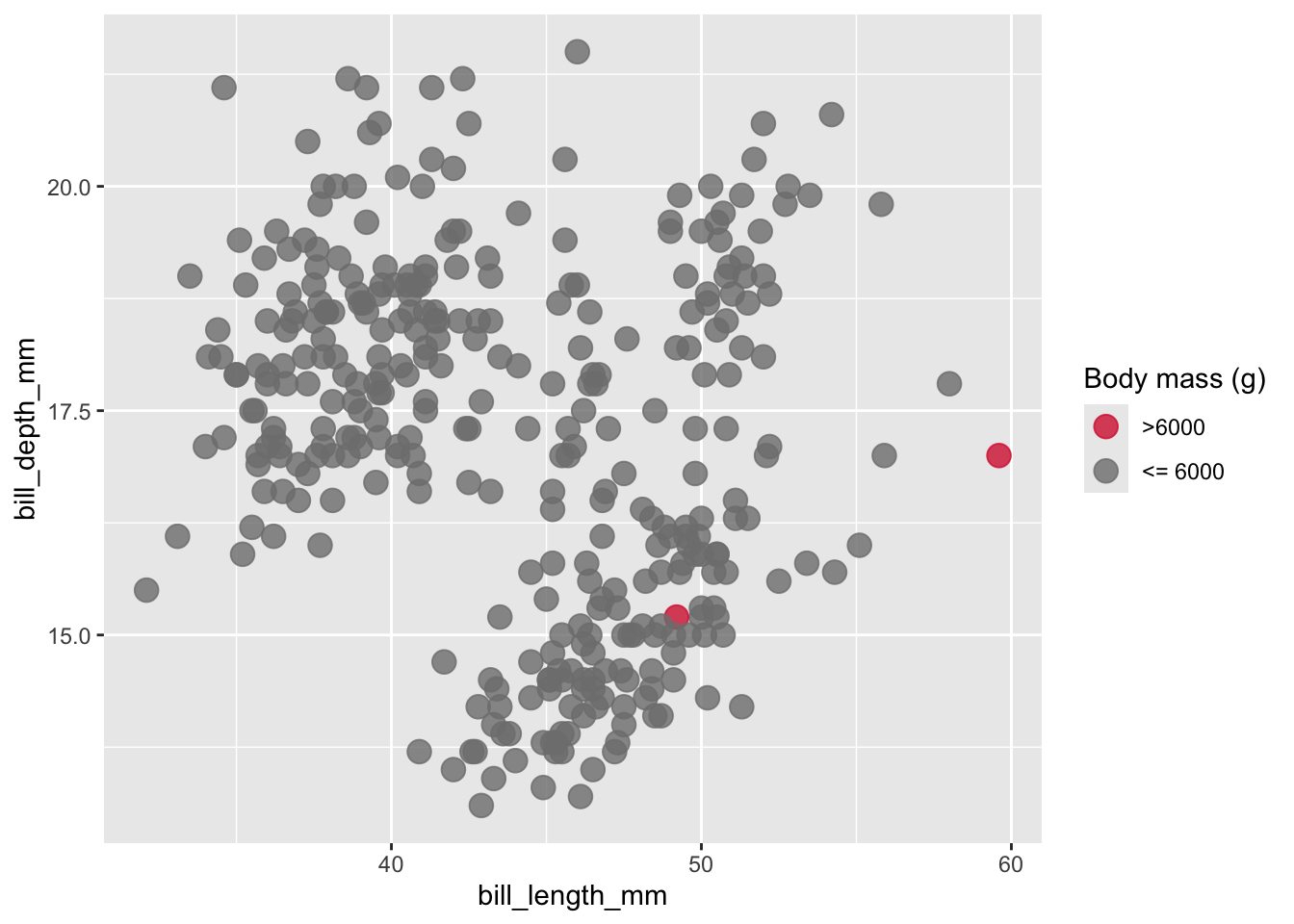
- Ex 2: color points based on criteria
# example 2 ----
penguins_ex2 <- penguins |>
  mutate(
    my_color = case_when(
      body_mass_g > 6000 ~ "#D7263D",
      TRUE ~ "gray50"
    )
  )

ggplot(penguins_ex2, aes(x = bill_length_mm, y = bill_depth_mm, color = my_color)) +
  geom_point(size = 4, alpha = 0.8) +
  scale_color_identity(guide = "legend",
                       name = "Body mass (g)",
                       labels = c(">6000", "<= 6000"))