Lecture 5.3 KEY – EDS 240

Note

This template follows lecture 5.3 slides. Please be sure to cross-reference the slides, which contain important information and additional context!

Setup

##~~~~~~~~~~~~~~~~~~~~~~~~~~~~~~~~~~~~~~~~~~~~~~~~~~~~~~~~~~~~~~~~~~~~~~~~~~~~~~
##                                    setup                                 ----
##~~~~~~~~~~~~~~~~~~~~~~~~~~~~~~~~~~~~~~~~~~~~~~~~~~~~~~~~~~~~~~~~~~~~~~~~~~~~~~

#..........................load packages.........................
library(tidyverse)
library(tigris)
library(sf)
library(RColorBrewer)
library(scales)

#.........................get shape data.........................
county_geo <- tigris::counties(class = "sf", cb = TRUE) |> # cb = TRUE to use cartographic boundary files
  
  # transform CRS to USA Contiguous Albers Equal Area Conic ----
  # see https://gis.stackexchange.com/questions/141580/which-projection-is-best-for-mapping-the-contiguous-united-states
  sf::st_transform("ESRI:102003")

#....................import precipitation data...................
precip_data <- read_csv(here::here("week5", "data", "NCEI-county-jan20-dec24-precip.csv"), 
                        skip = 4)

##~~~~~~~~~~~~~~~~~~~~~~~~~~~~~~~~~~~~~~~~~~~~~~~~~~~~~~~~~~~~~~~~~~~~~~~~~~~~~~
##                               data wrangling                             ----
##~~~~~~~~~~~~~~~~~~~~~~~~~~~~~~~~~~~~~~~~~~~~~~~~~~~~~~~~~~~~~~~~~~~~~~~~~~~~~~
     
##~~~~~~~~~~~~~~~~~~~~~~~~~~~~
##  ~ wrangle geometries  ----
##~~~~~~~~~~~~~~~~~~~~~~~~~~~~

county_geo_wrangled <- county_geo |>
  
  # clean up col names ----
  janitor::clean_names() |>
  
  # rename county & state cols ----
  rename(county = namelsad, state = state_name) |>
  
  # keep only 50 US states (minus AK & HI) ----
  filter(state %in% state.name) |> # `state.name` is a build-in vector of the 50 US States
  filter(!state %in% c("Alaska", "Hawaii")) |> 
  
  # capitalize "city" in county names (so that it matches those in `precip_data`) ----
  mutate(county = str_replace(string = county, pattern = " city", replacement = " City"))

##~~~~~~~~~~~~~~~~~~~~~~~~~~~~~~~~~~~~
##  ~ wrangle precipitation data  ----
##~~~~~~~~~~~~~~~~~~~~~~~~~~~~~~~~~~~~

precip_wrangled <- precip_data |>
  
  # clean up col names ----
  janitor::clean_names() |>
  
  # rename county col ----
  rename(county = name) |>
  
  # keep only US states (this will filter out DC) ----
  filter(state %in% state.name) |> 
  
  # update county name so that it matches the spelling in `county_geo` df ----
  mutate(county = str_replace(string = county, pattern = "Dona Ana County", replacement = "Doña Ana County")) |>
  
  # coerce precip & 20th centruy avg from chr to numeric ----
  mutate(value = as.numeric(value),
         x1901_2000_mean = as.numeric(x1901_2000_mean)) |>
  
  # calculate % change in precip from 20th century avg ----
  mutate(perc_change = ((value - x1901_2000_mean)/x1901_2000_mean)*100) |>
  
  # select, rename, reorder cols ----
  select(id, state, county, mean_1901_2000 = x1901_2000_mean, precip = value, perc_change, anomaly_1901_2000_base_period)

##~~~~~~~~~~~~~~~~~~
##  ~ join dfs  ----
##~~~~~~~~~~~~~~~~~~

# join dfs (be sure to join precip TO sf object, not the other way around; see https://github.com/tidyverse/ggplot2/issues/3936 & https://map-rfun.library.duke.edu/032_thematic_mapping_geom_sf.html)) -------
joined_precip_geom <- full_join(county_geo_wrangled, precip_wrangled)

Create map

Create base map

# create base map ----
base_map <- ggplot(joined_precip_geom) +
  geom_sf(aes(fill = perc_change), linewidth = 0.1) +
  labs(title = "5-year precipitation compared with the 20th century average",
       subtitle = "January 2020 - December 2024",
       caption = "Source: National Centers for Environmental Information") +
  theme_void() +
  theme(
    legend.position = "bottom",
    legend.title = element_blank(),
    plot.caption = element_text(face = "italic",
                                margin = margin(t = 10, r = 5, b = 0, l = 0))
  )

base_map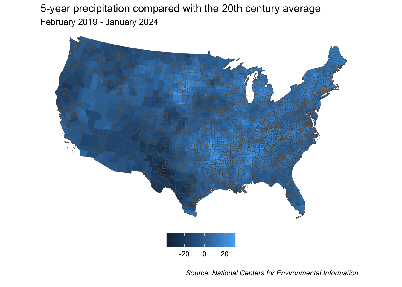

Create an unclassed map

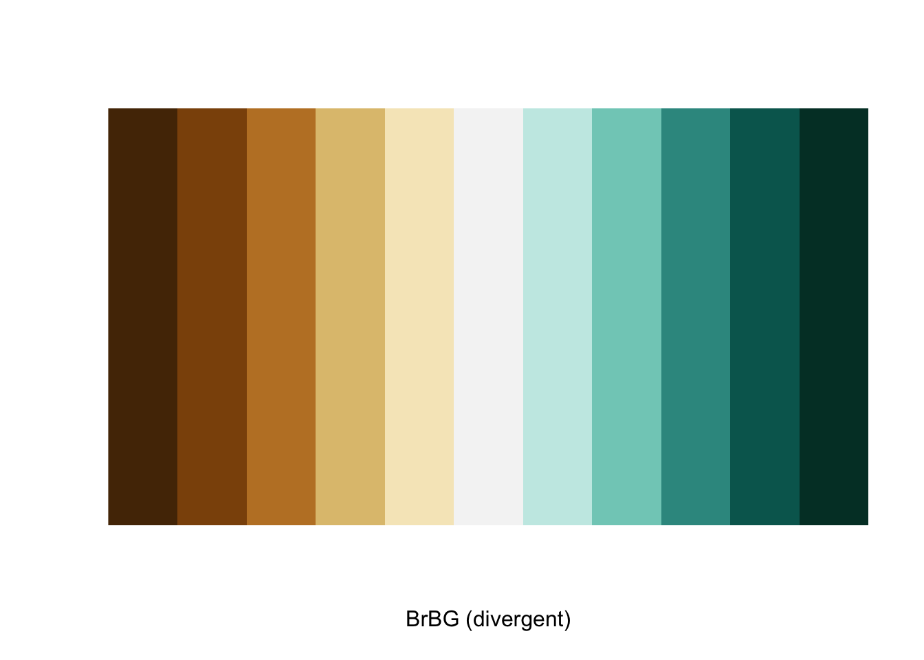
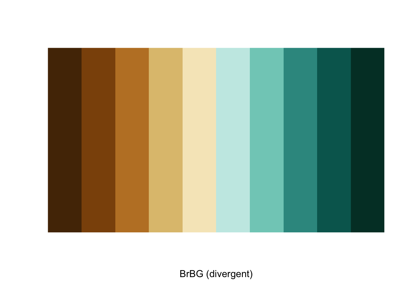
create color palette

# preview palette ----
RColorBrewer::display.brewer.pal(n = 11, name = "BrBG")

# save HEX codes as vector ----
my_brew_palette11 <- RColorBrewer::brewer.pal(n = 11, name = "BrBG")

build map

# create unclassed map ----
base_map + 
  scale_fill_gradientn(colors = my_brew_palette11,
                       labels = scales::label_percent(scale = 1),
                       breaks = scales::breaks_width(width = 10),
                       values = scales::rescale(x = c(-40, 0, 20))) +
  guides(fill = guide_colorbar(barwidth = 25, barheight = 0.75))

Create a classed map

create color palette

# preview palette ----
RColorBrewer::display.brewer.pal(n = 10, name = "BrBG")

# save HEX codes as vector ----
my_brew_palette10 <- RColorBrewer::brewer.pal(n = 10, name = "BrBG")

build map

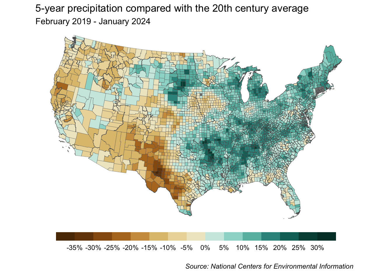
# classed map with default bins ----
base_map + 
  scale_fill_stepsn(colors = my_brew_palette10,
                    labels = scales::label_percent(scale = 1)) +
  guides(fill = guide_colorsteps(barwidth = 25, barheight = 0.75))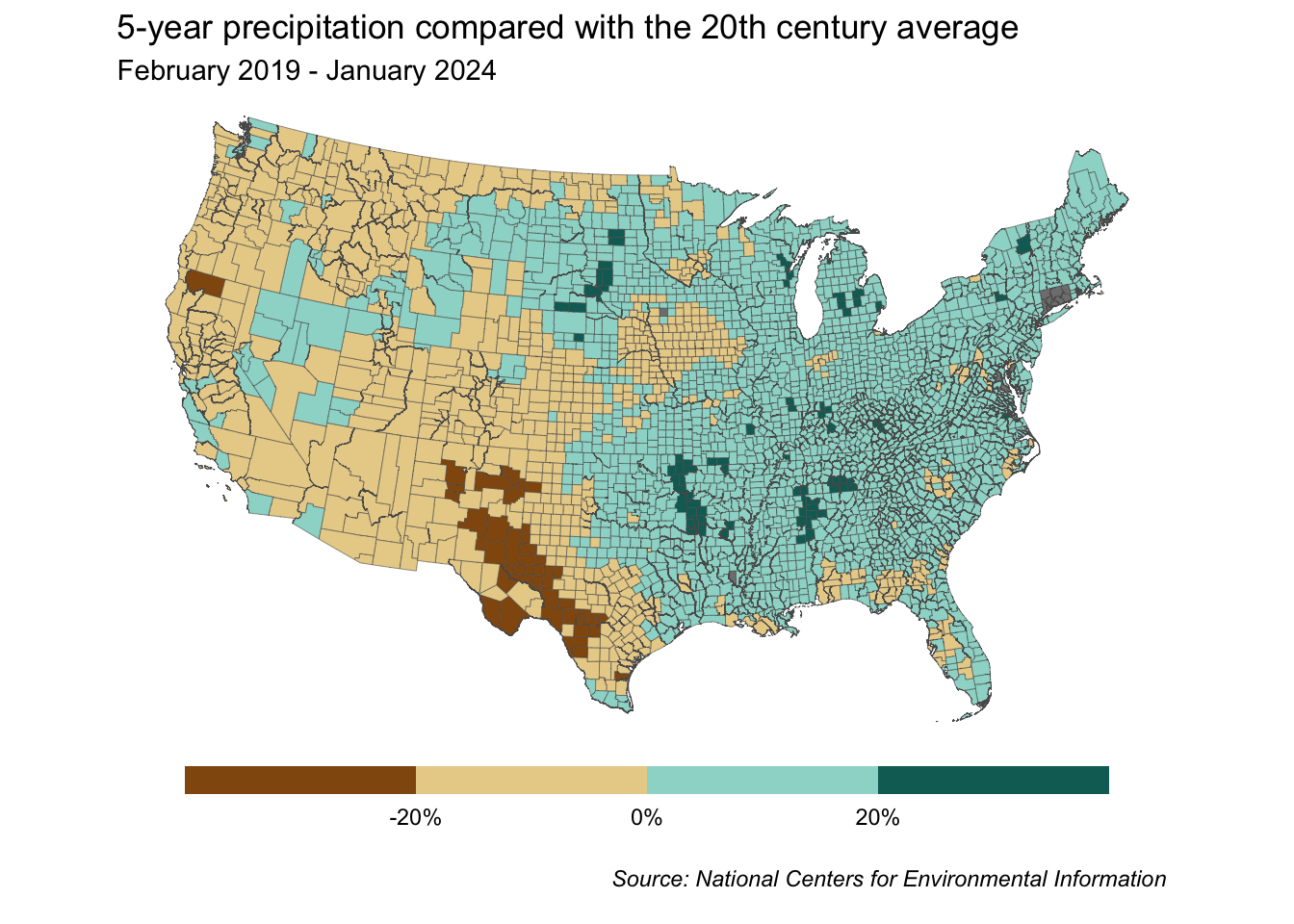

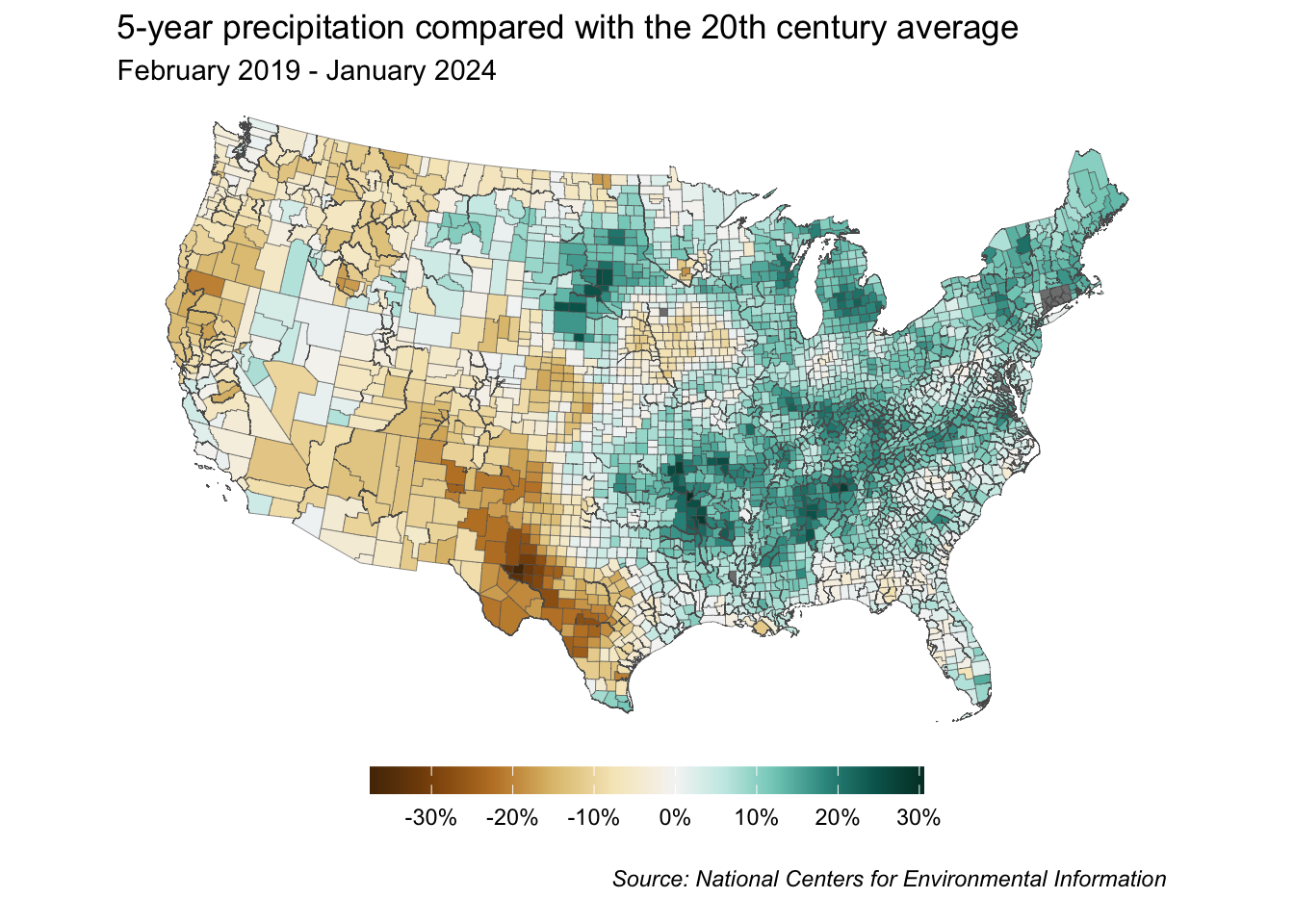
# bins have width of 10 ----
base_map + 
  scale_fill_stepsn(colors = my_brew_palette10,
                    labels = scales::label_percent(scale = 1),
                    breaks = scales::breaks_width(width = 10),
                    values = scales::rescale(x = c(-40, 0, 20))) +
  guides(fill = guide_colorsteps(barwidth = 25, barheight = 0.75))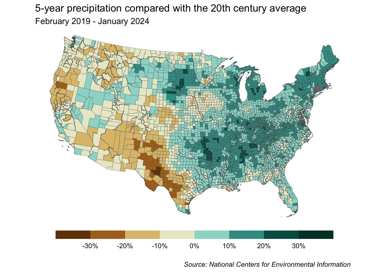

# bins have width of 5 ---
base_map + 
  scale_fill_stepsn(colors = my_brew_palette10,
                    labels = scales::label_percent(scale = 1),
                    breaks = scales::breaks_width(width = 5),
                    values = scales::rescale(x = c(-40, 0, 20))) + 
  guides(fill = guide_colorsteps(barwidth = 25, barheight = 0.75))